Solver

GMPT, October 2024

---

Macondo offers multiple solver options, including the FDTD 3D Solver, EME 3D Solver, and FDE Solver. Users can select the appropriate solution based on their simulation needs and specific requirements.

---

FDTD 3D Solver

The FDTD 3D Solver uses the Finite-Difference Time-Domain algorithm to rigorously solve the full-vector Maxwell's equations. Maxwell's Curl Equations： $$\mathrm{\nabla }\times \mathbf{\text{H}}=\frac{\mathrm{\partial }\mathbf{\text{D}}}{\mathrm{\partial }t}+\mathbf{\text{J}}\backslash nabla\; \backslash times\; \backslash textbf\{H\}\; =\; \backslash frac\{\backslash partial\; \backslash textbf\{D\}\}\{\backslash partial\; t\}\; +\; \backslash textbf\{J\}$$

$$\mathrm{\nabla }\times \mathbf{\text{E}}=-\frac{\mathrm{\partial }\mathbf{\text{B}}}{\mathrm{\partial }t}-{\mathbf{\text{J}}}_m\backslash nabla\; \backslash times\; \backslash textbf\{E\}\; =\; -\backslash frac\{\backslash partial\; \backslash textbf\{B\}\}\{\backslash partial\; t\}\; -\; \backslash textbf\{J\}\_m$$

Finite-Difference Time-Domain (FDTD) Iterative Equations：

$$E_x^{n+1}(i+\frac{1}{2},j,k)=C_1\cdot E_x^{n+1}(i+\frac{1}{2},j,k)E^\{n+1\}\_x(i+\backslash frac\{1\}\{2\},j,k)\; =\; C\_1\backslash cdot\; E^\{n+1\}\_\{x\}(i+\backslash frac\{1\}\{2\},j,k)$$ $$+C_2\cdot [H_z^{n+\frac{1}{2}}(i+\frac{1}{2},j+\frac{1}{2},k)-H_z^{n+\frac{1}{2}}(i+\frac{1}{2},j-\frac{1}{2},k)]+C\_2\backslash cdot\; \backslash left[H^\{n+\backslash frac\{1\}\{2\}\}\_\{z\}(i+\backslash frac\{1\}\{2\},j+\backslash frac\{1\}\{2\},k)-H^\{n+\backslash frac\{1\}\{2\}\}\_\{z\}(i+\backslash frac\{1\}\{2\},j-\backslash frac\{1\}\{2\},k)\backslash right]$$ $$-C_3\cdot [H_y^{n+\frac{1}{2}}(i+\frac{1}{2},j,k+\frac{1}{2})-H_y^{n+\frac{1}{2}}(i+\frac{1}{2},j,k-\frac{1}{2})],-C\_3\backslash cdot\; \backslash left[H^\{n+\backslash frac\{1\}\{2\}\}\_\{y\}(i+\backslash frac\{1\}\{2\},j,k+\backslash frac\{1\}\{2\})-H^\{n+\backslash frac\{1\}\{2\}\}\_\{y\}(i+\backslash frac\{1\}\{2\},j,k-\backslash frac\{1\}\{2\})\backslash right]\; ,$$ $$C_1=\frac{2\epsilon -\sigma \mathrm{\Delta }t}{2\epsilon +\sigma \mathrm{\Delta }t},C_2=\frac{2\mathrm{\Delta }t}{(2\epsilon +\sigma \mathrm{\Delta }t)\cdot \mathrm{\Delta }y},C_3=\frac{2\mathrm{\Delta }t}{(2\epsilon +\sigma \mathrm{\Delta }t)\cdot \mathrm{\Delta }z},C\_1\; =\; \backslash frac\{2\backslash varepsilon-\backslash sigma\backslash Delta\; t\}\{2\backslash varepsilon+\backslash sigma\backslash Delta\; t\},\; C\_2\; =\; \backslash frac\{2\backslash Delta\; t\}\{(2\backslash varepsilon+\backslash sigma\backslash Delta\; t)\backslash cdot\backslash Delta\; y\},\; C\_3\; =\; \backslash frac\{2\backslash Delta\; t\}\{(2\backslash varepsilon+\backslash sigma\backslash Delta\; t)\backslash cdot\backslash Delta\; z\},$$

---

Features of the FDTD (Finite-Difference Time-Domain) Solver

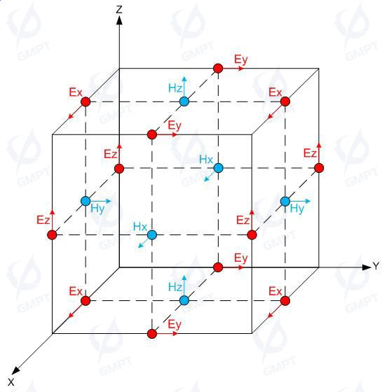
Based on the spatiotemporal relationship, the Yee cell discretization alternately iterates the electromagnetic properties at each time step and spatial step. By injecting a pulse excitation, a single simulation can capture the broadband response of the light source. This is a primary technical approach for studying wave optics and electromagnetic wave problems.

• The dispersive FDTD solver, combined with material refractive index fitting algorithms, can accurately simulate the dispersive properties of devices.

• The non-dispersive FDTD solver uses a dielectric material model, considering only the refractive index at a single frequency, allowing for fast simulation of the electromagnetic properties of passive devices.

Yee Cell：

Mode Propagation Evolution in Optical Waveguides：

EME 3D Solver

The EME 3D solver is based on the eigenmode expansion algorithm and mode propagation algorithm, used for analyzing and optimizing optical waveguide devices and structures.

---

Features of the EME (EigenMode Expansion) Algorithm

The simulation region is divided into multiple YZ-plane slices along the X direction, where the modes and overlap integrals of each slice are calculated. Using the mode propagation and eigenmode expansion algorithms, the S-parameters of the slices and ports are obtained. The calculation speed and accuracy mainly depend on the number of modes calculated for the ports and slices.

• EME 3D solver: Designed specifically for waveguide device simulations, it enables fast simulations for large devices in the propagation direction and serves as a convenient tool for designing waveguide devices.

FDE Solver

The FDE solver is based on the Finite-Difference Eigenmode (FDE) algorithm, allowing users to analyze waveguide mode distribution, effective refractive index, mode field polarization, and waveguide loss.

---

Features of the FDE (Finite Difference EigenMode) Algorithm

Based on the structured discrete mesh and refractive index conformal algorithm using finite differences, it can quickly solve for the mode distribution and effective refractive index of the spatial cross-section.

• FDE Solver: A simulator specifically designed for 2D mode calculations of waveguides. The FDE Analysis feature allows for quick mode scanning at different frequencies. Combined with the NP Density Import function, it can solve for electro-optic response characteristics resulting from refractive index perturbations.

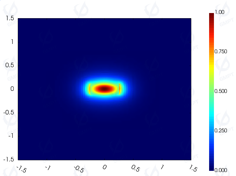
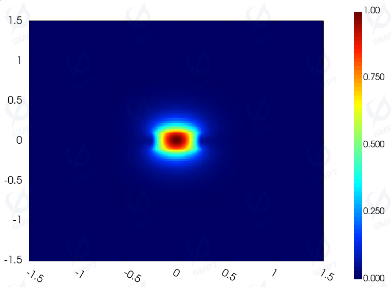
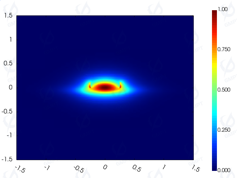
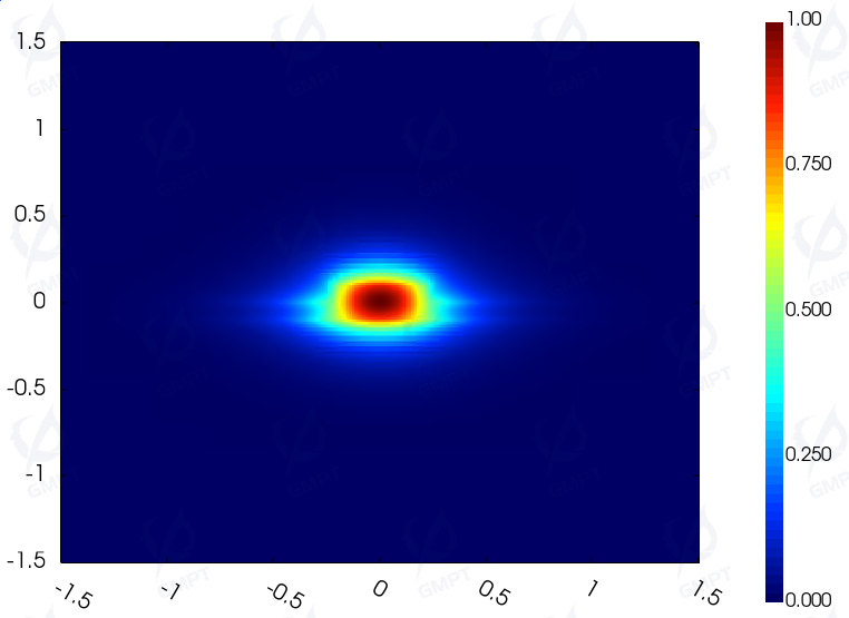
Mode Field Distribution：

 （a）Fundamental mode electric field component/magnetic field component of a straight waveguide

 （b）Fundamental mode electric field component/magnetic field component of a ridge waveguide

Conformal Mesh and Meshing Techniques

Conformal mesh and meshing techniques are fundamental conditions for ensuring the accuracy of the Finite-Difference Time-Domain (FDTD) algorithm.

---

Features of the Conformal Mesh Algorithm

The conformal mesh primarily addresses calculation errors that occur when there are abrupt changes in the refractive index of materials. It allows for precise and stable results while using fewer computational resources.

The methods used by the software to handle meshes with abrupt changes in material refractive index include:

• Advanced Conformal Method: Derived from physical equations, this method integrates the advantages of various conformal handling techniques and is finely tuned to solve the issue of large numerical errors at the material interfaces between different media in gradual transition meshes.
• Conformal Method: A volume-weighted averaging method. While it lacks a rigorous physical foundation, it is simple and accurate, making it suitable for most scenarios.
• Staircase Method: A traditional stepped refractive index mesh that is simple and fast but has significant numerical errors.

The software provides the following meshing methods for handling scenes and geometries:

• Uniform Mesh: Divides the entire simulation region into uniform-width meshes.
• Non-Uniform Mesh (Gradual Transition Mesh): Divides the region with uniform meshes based on the relationship between refractive index and wavelength, and applies gradual transition meshes at interfaces where the refractive index changes abruptly.
• Submesh: Adds submesh regions within an already meshed area for localized processing.

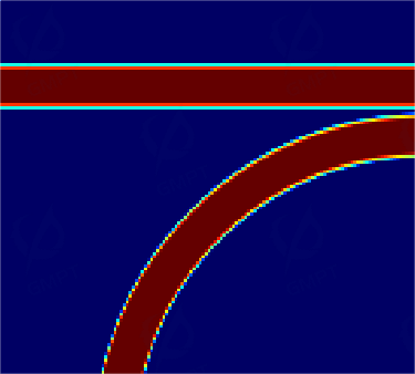
Conformal Mesh Division for Straight and Curved Waveguides:

Boundary Conditions

At the boundaries of the solution region, boundary conditions are used to represent different real-world spatial characteristics. The software has built-in boundary conditions, which include:

• Metal: A total reflection boundary condition that confines electromagnetic wave energy within the simulation region. It is commonly used as a boundary condition for mode calculations.
• PML (Perfectly Matched Layer): An absorbing boundary condition that uses multi-layered, varying scale dielectric layers as a matching absorption layer to suppress the reflection of the optical field energy, thereby achieving the absorption of incident light. It is commonly used in FDTD simulations to model an infinite simulation region or to eliminate reflection effects.
• Bloch: A periodic boundary condition primarily used for cases of oblique incidence of plane waves on an infinite plane. It addresses the issue of phase discontinuity at the boundaries for plane wave sources.

Advanced Settings for Solver Computational Efficiency

To improve simulation efficiency, the software includes built-in solver calculation settings:

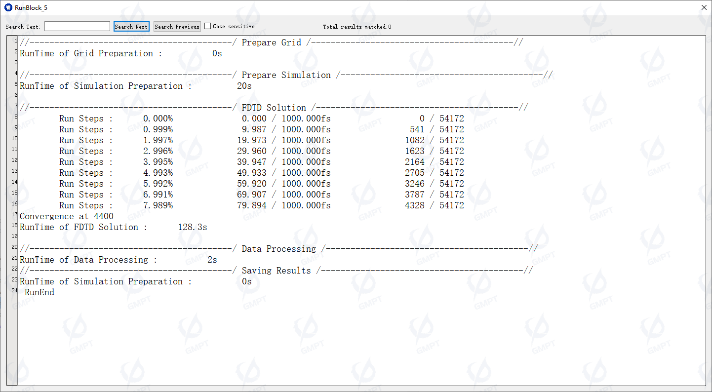
• Auto Finish Convergence/Divergence Criteria: Determines the interaction between light and the structure by monitoring the energy decay process of the optical field within the simulation region, to assess whether the simulation has been completed.

• Resources Parallel Computing Resource Management: By setting the number of computational threads for the CPU, it leverages parallel computing algorithms to enhance simulation efficiency.

FDTD Iteration Early Convergence, Run Log: