Using Rayzen Software to Simulate a Night Vision Compatible LCD Backlight Module

GMPT, October 2024

1. Introduction

Backlight modules are crucial components in LCD technology, providing a uniform and sufficient light source for the display. In aviation LCD applications, not only are low power consumption, high brightness, high reliability, and sunlight readability required, but compatibility with night vision imaging systems is also essential. Standard cockpit lighting and information displays emit high levels of radiation in the near-infrared band, which can activate the automatic gain control system in night vision devices, decreasing sensitivity and impairing pilots' night vision ability${}^{[1]}^\{[1]\}$.
To address this challenge, domestic LCD devices commonly use a dual-mode backlight system to enhance night vision compatibility. In non-night vision environments, high-efficiency white LED lights serve as the backlight source, providing bright displays with low power consumption. In night vision environments, they switch to OGB (orange-green-blue) LED lights, composed of blue, green, and orange (wavelength range 590-610 nm) chips. This combination effectively reduces near-infrared radiation, lowering night vision brightness and ensuring night vision devices function correctly.
Backlight modules are divided into direct-type and edge-lit based on the light entry method. Direct-type backlight modules provide uniform light output and high light extraction efficiency but are bulky, making them suitable for larger products. Edge-lit backlight modules offer a thinner structure by placing the light source on the side of the light guide plate, which aligns with the trend towards thinner displays in LCD technology. However, edge-lit modules have higher manufacturing complexity and relatively lower light uniformity and utilization rates. For small and medium-sized LCD modules, edge-lit backlight technology is mature, making the modules thinner and more convenient to use${}^{[2]}^\{[2]\}$.
To further enhance display quality and night vision compatibility, this study simulates an edge-lit backlight module using white and OGB LEDs. With Rayzen, a backlight model is constructed, and simulation phenomena are analyzed theoretically to assess illumination uniformity and validate model practicality and efficiency.

2. Structure of the Edge-lit Backlight Module

In the display panel industry, key performance indicators include illumination, uniformity, color accuracy, and viewing angle, all directly impacting the visual experience and overall performance. Among these, illumination and uniformity are primarily determined by the backlight module. An edge-lit backlight module consists of a light source, light guide plate, and a series of optical films.
The light guide plate is the core component of the backlight module, directing the light emitted from the source in the desired direction through total reflection and scatter dot arrangements on its bottom surface. The geometric shape and material selection of the light guide plate directly influence the brightness, light extraction efficiency, and uniformity of the emitted light.
To improve light extraction efficiency, reflective films are placed on the non-light-emitting surfaces of the light guide plate, reflecting scattered light back into the plate for reuse. Unlike mirror reflection, the reflective film slightly scatters the light.
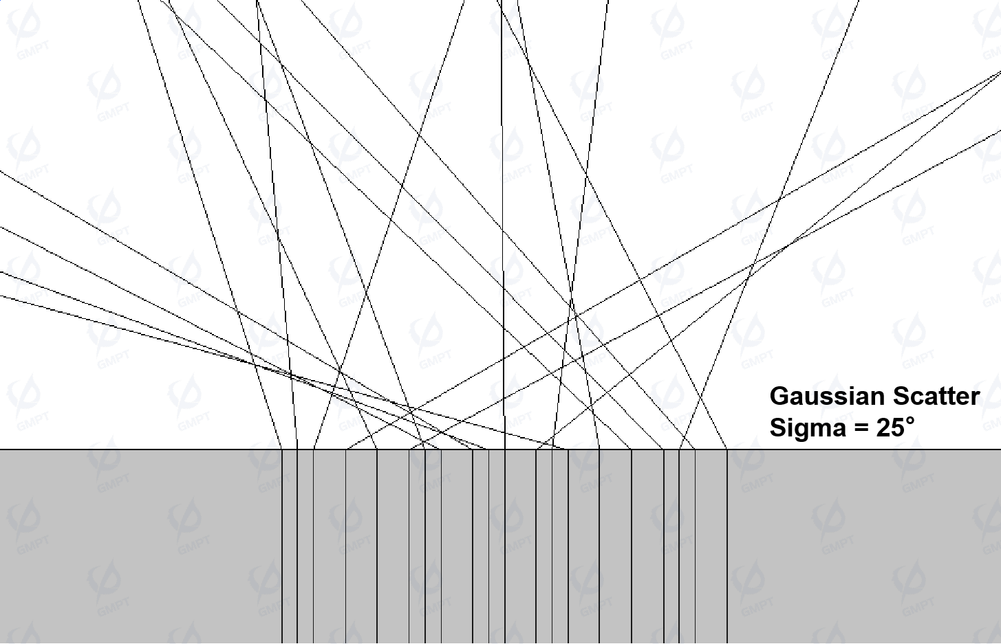
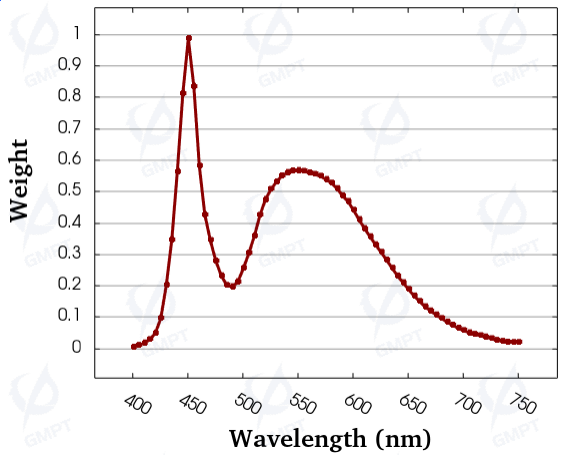
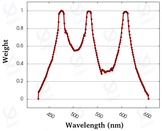
Improper size, shape, and arrangement of scatter dots can lead to bright spots, lines, and diffraction patterns. To prevent this, a diffuser film is added before the light enters the LCD, scattering the light to eliminate bright spots, lines, and diffraction fringes, making the position and direction distribution of emitted light more uniform. As shown in Figure 1, this diffuser has a scattering property approximated by Gaussian scattering in this study.

Figure 1. Gaussian Light Diffusion

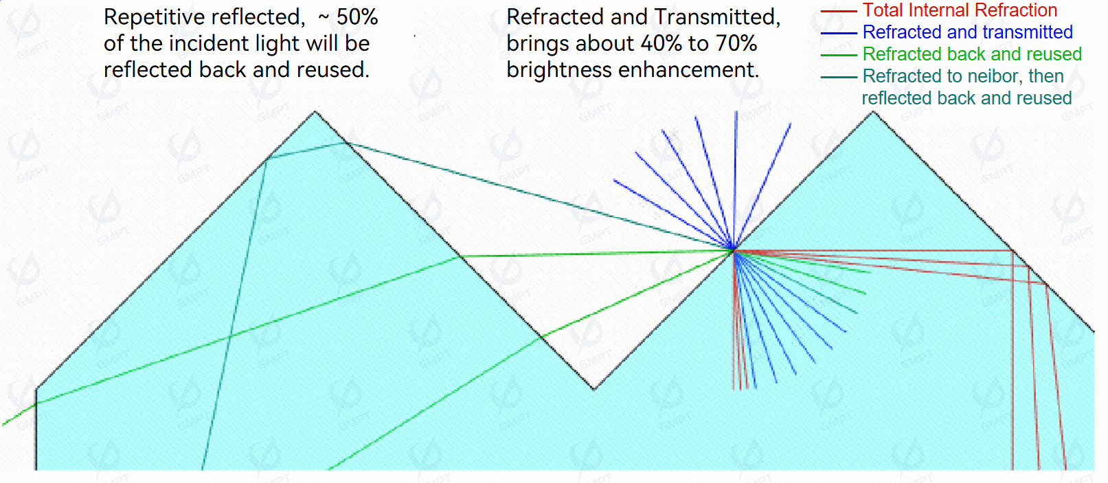
After passing through the diffuser, the angle of the light beam expands, reducing the brightness of the LCD. Thus, a brightness enhancement film is added to redirect the light, increasing utilization. These films usually feature prismatic microstructures on their surfaces, using total internal reflection to redirect wide-angle light back to the enhancement film, increasing front brightness and reducing energy loss. Backlight modules typically use two crossed prismatic films for greater brightness. Figure 2 illustrates the structure and principle of the brightness enhancement film${}^{[3]}^\{[3]\}$.

• Light entering the enhancement film at a wide angle undergoes total internal reflection, returning to the surface.
  
• Light entering at an angle just breaking total reflection refracts once, with most light focused within a 70° range, improving front brightness.
  
• Lowering the light’s angle further results in two or three refractions into the next prism.
  

Figure 2. Schematic of Brightness Enhancement Film Principle

3. Design Concept of the Backlight Module

3.1 Overview of Backlight Module Design

As the only light source for LCDs, the backlight module’s performance directly impacts optical efficiency and night vision compatibility. To achieve high brightness and night vision compatibility, precise and efficient optical design is essential. Using a 10.4-inch LCD module as an example, the design process is analyzed from the perspective of selecting the backlight lamps (white + OGB lights) and the light guide plate.

3.2 Dual-Mode Light Source Strategy

To meet the night vision compatibility requirements of GJB 1394-1992 II Type B standards, white and OGB lights are used. In daylight mode, both lights work to enhance brightness and color range; in night mode, only the OGB lights work to eliminate interference in the near-infrared band, meeting night vision compatibility requirements. The light source enters through the two long edges of the light guide plate, with 98 LEDs in total. Fifty white LEDs, each with a luminous flux of 124 lm and dimensions of 3x3 mm, and 48 OGB LEDs, each with a flux of 3.8 lm and dimensions of 2.8x3.5 mm, alternate along each edge, with spacing of 4.4 mm. The distance from the emitting surface of the white LEDs to the entry of the light guide plate is 0.98 mm, and 0.95 mm for the OGB LEDs${}^{[4]}^\{[4]\}$.
Currently, Rayzen supports using radiant flux as the unit for illumination calculation. The following formula converts luminous flux to radiant power for simulation:

$${\mathrm{\Phi }}_v=P_e\cdot K_m\cdot {\int }_{{\lambda }_0}^{\lambda }V(\lambda )d\lambda (1)\backslash Phi\_v=P\_e\backslash cdot\{K\_m\}\backslash cdot\backslash int\_\{\backslash lambda\_0\}^\backslash lambda\; V(\backslash lambda)d\backslash lambda\; \backslash qquad(1)$$

where:
${\mathrm{\Phi }}_v\backslash Phi\_v$ = luminous flux, in lumens (lm).
$K_{m}K\_m$ = maximum luminous efficacy, typically 683 lm/W.
$P_{e}P\_e$ = radiant power at wavelength λ, in watts (W).
$V(\lambda )V(\backslash lambda)$ = spectral luminous efficiency function.

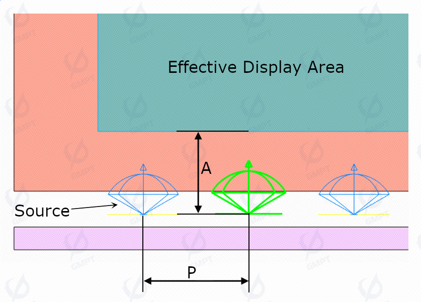
In edge-lit backlight design, improper LED layout can lead to brightness and darkness variations along the light entry side of the light guide plate, known as HotSpot effect. The A/P index usually assesses the likelihood of HotSpot occurrence. As shown in Figure 3, A is the distance from the light-emitting surface to the active area of the LCD, and P is the pitch between light sources. Table 1 shows A values, P values, and HotSpot assessment for white and OGB lights. The LED layout in this study does not produce visible HotSpot effects.

• A/P<0.5 results in significant HotSpot effect, correctable with dot design but unremovable.
  
• 0.5≤A/P≤0.7 produces slight HotSpot effect, improvable with dot design.
  
• A/P>0.7 produces no visible HotSpot effect.
  

Figure 3. Schematic of A and P Values in Backlight Design

Table 1 White and OGB Layout and HotSpot Evaluation

Type	A Value (mm)	P Value (mm)	A/P	HotSpot
White Light	3.48	4.4	0.79	No
OGB Light	3.45	4.4	0.78	No

3.3 Structural Design of the Light Guide Plate in Edge-lit Backlight Modules

The thin design of LCD modules holds critical significance, especially in specialized display applications, where lightweight designs considerably enhance the endurance of airborne equipment. As the backlight module comprises approximately 70% of the LCD module's thickness and weight, reducing its size is naturally pivotal for achieving a thinner LCD display.
In this design, considering the light-emitting surface height of the OGB color light set to 3.5 mm, we evaluate the plate thickness. Using a light guide plate thinner than the light's height may achieve a more compact form, but it results in a significant loss of light efficiency. A light guide plate that is slightly thicker than the LED height maintains a good balance, partially sacrificing light efficiency while meeting the design goal for thinness. Therefore, we selected a thickness of 4 mm for the light guide plate to balance both light efficiency and thinness.
Moreover, the dot distribution on the light guide plate is another essential factor in optimizing the backlight module’s performance. Rayzen supports parameterized dot design, including shape parameters, such as radius and sag height for hemispherical dots, and arrangement parameters, like spacing in uniform layouts. Understanding the trends in light transmission efficiency and uniformity with parameter changes, and analyzing their causes, provides guidance for dot distribution design.

Figure 4. Effect of Increasing Dot Spacing on Received Power (left), Contrast (middle), and Mean Deviation (right)

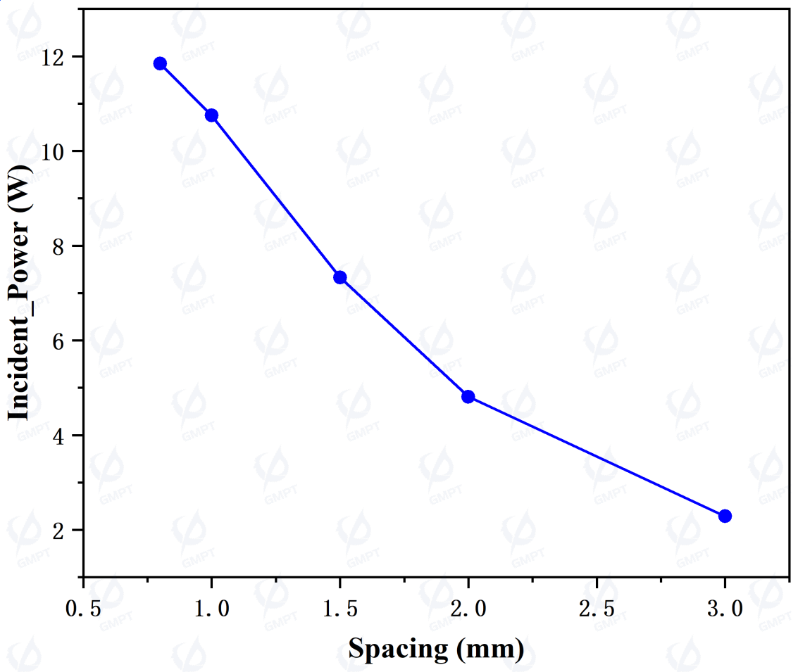
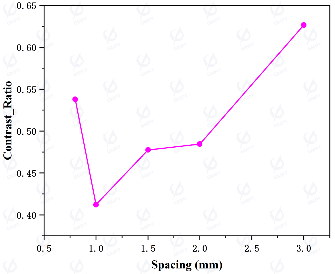
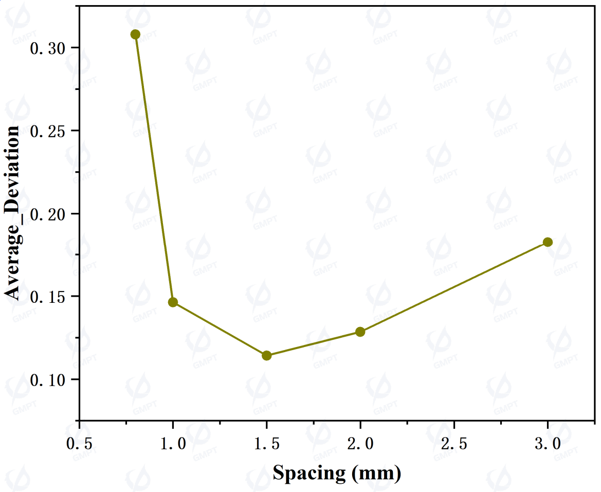
Initially, we analyze the relationship between dot spacing and output power, contrast, and mean deviation, assuming that each dot has identical spacing in both directions. As shown in Figure 4, 1. As spacing increases, output power decreases. With fewer dots, the probability of total internal reflection at the bottom of the light guide plate increases, resulting in more power absorbed within the material. 2. As spacing increases, contrast initially decreases, then increases, indicating an initial improvement in uniformity followed by a decline. Each dot scatters light similarly; fewer dots near the light source reduce light extraction, thereby decreasing peak output power and increasing uniformity. As spacing further increases, light scattering from each dot becomes more isolated, causing alternating bright and dark regions on the output surface, lowering uniformity. Fewer emitted rays also reduce statistical convergence, making uniformity metrics more susceptible to outliers. 3. As spacing increases, mean deviation initially decreases, then increases. Unlike contrast (uniformity), mean deviation focuses more on the relative proportion of data with higher deviation. Thus, the initial decrease in mean deviation is due to improved uniformity from fewer dots near the light source; later, deviation increases as statistical convergence diminishes. Based on this analysis, setting dot spacing at 1 mm is a reasonable choice.

Figure 5. Effect of Increasing Dot Radius and Height Proportionally on Received Power (left), Contrast (middle), and Mean Deviation (right)

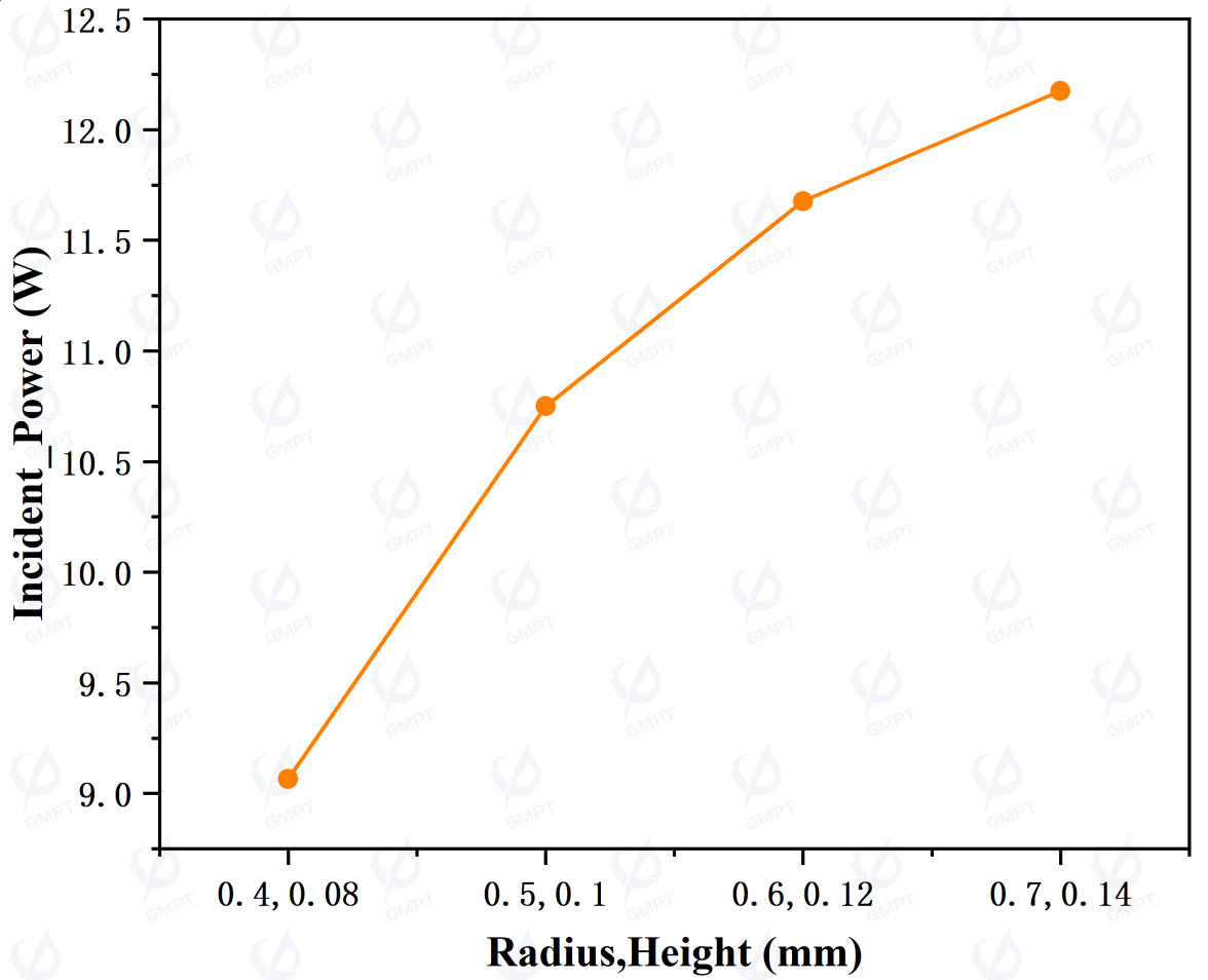
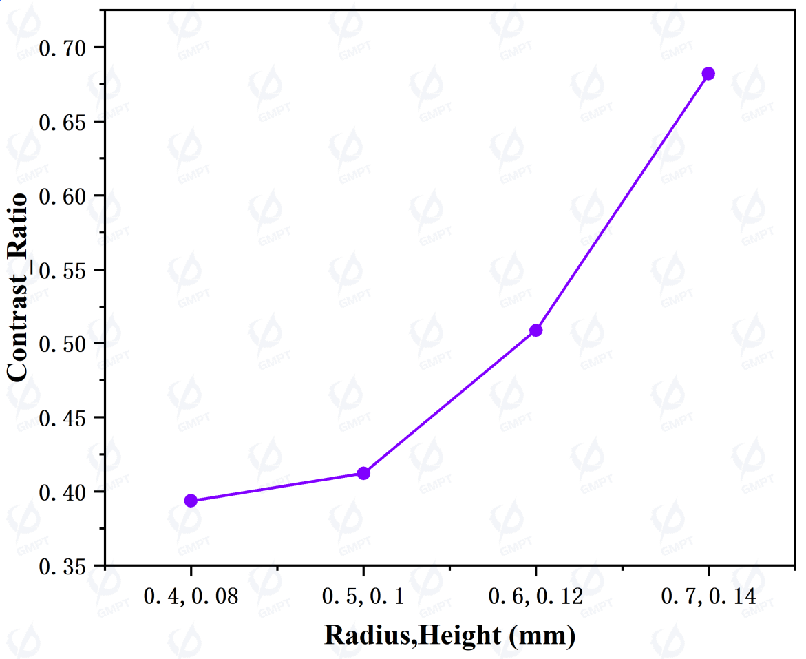
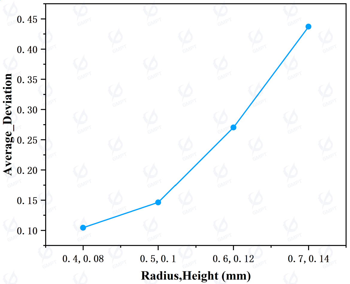
Next, we analyze the relationship between dot size and the above metrics, maintaining proportionality between dot radius and sag height for uniform dot size. As shown in Figure 5, as dot size increases, output power increases by approximately 35%, uniformity decreases by about 70%, and mean deviation rises by about 330%. This increase in dot size significantly enhances light extraction efficiency near the light source. Based on this data, a dot radius of 0.5 mm and height of 0.1 mm provides a balance, enhancing light extraction efficiency while maintaining good convergence and uniformity.

Figure 6. Effect of Increasing Dot Height on Received Power (left), Contrast (middle), and Mean Deviation (right)

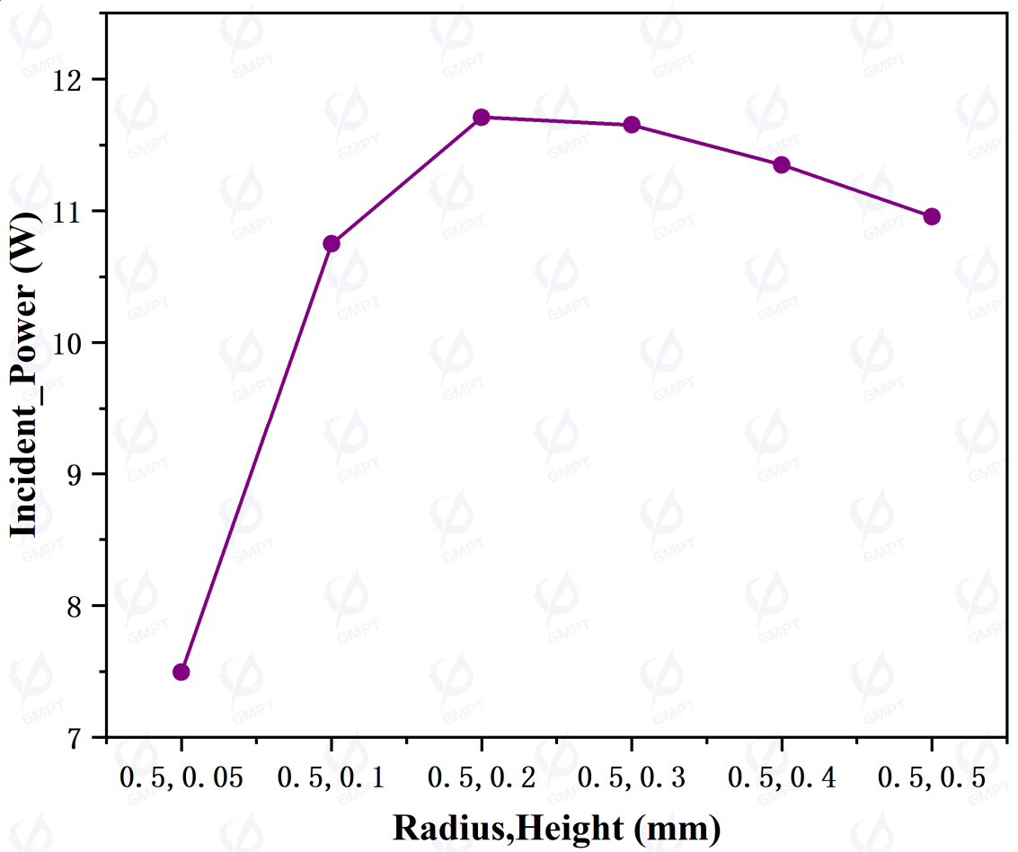
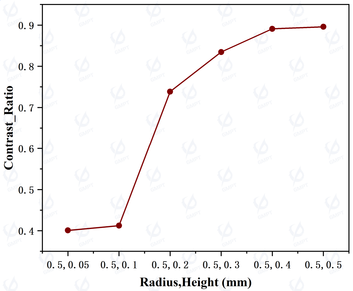
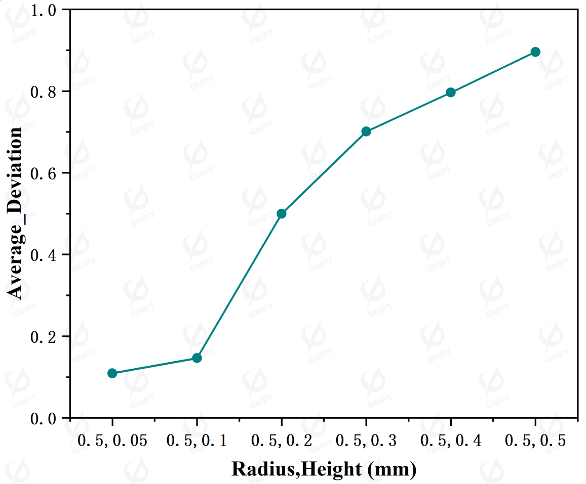
Finally, we analyze the relationship between dot radius and varying sag height ratios with these metrics. We assume each dot radius to be 0.5 mm and evenly distributed. As shown in Figure 6, as sag height increases, output power initially increases, then slightly decreases, while uniformity decreases by about 110%, and mean deviation increases by about 750%. When sag height is set to 0.05 mm, the dots' disruption of total internal reflection is weak, keeping significant light within the light guide plate, thereby reducing light extraction efficiency. Increasing sag height from 0.05 mm to 0.1 mm significantly enhances the dots' ability to disrupt total internal reflection, increasing the extraction proportion in the input side region. This reduces the light reaching the center, leading to increased contrast and mean deviation. Based on this data, a sag height of 0.1 mm provides a significant boost in extraction power while ensuring adequate uniformity and convergence.${}^{[5]}^\{[5]\}$

3.4 Theoretical Analysis of Dot Spacing Arrangement

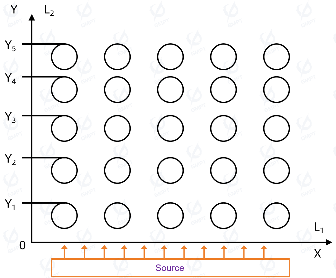
As light enters from both sides of the light guide plate, total internal reflection occurs, and light scatters when it encounters a dot, with some light emitted from the front. The total light flux decreases continuously, necessitating denser dot spacing for uniform front illumination. As illustrated in Figure 7, the light source is distributed along the X-axis, and dots are arranged at equal intervals along the X-direction with each row containing an equal number of dots. The base of the light guide plate has a length of $L_{1}L\_1$ and a width of $L_{2}L\_2$. In the Y direction, the guide plate is divided into n rectangles along coordinates $Y_{1}Y\_1$, $Y_{2}Y\_2$, $Y_{3}Y\_3$ ... $Y_{n}Y\_n$.${}^{[6]}^\{[6]\}$

Figure 7. Dot Distribution Model of the Light Guide Plate

Assuming no loss and that light enters the guide plate with uniform intensity, the total flux from one side is $\mathrm{\Phi }\backslash Phi$, and each row’s dot scattering coefficient is $kk$. For single-side illumination, the front illumination is:

$$B=\frac{k\mathrm{\Phi }}{S_1}=\frac{k\mathrm{\Phi }}{Y_1{L}_1}(2)B\; =\; \backslash frac\{k\; \backslash Phi\}\{S\_1\}=\backslash frac\{k\backslash Phi\}\{Y\_1L\_1\}\; \backslash qquad(2)$$

The flux conservation formula for regions ($0-Y_{1}0-Y\_1$) and ($Y_1-Y_{2}Y\_1-Y\_2$) is:

$$\frac{k\mathrm{\Phi }}{Y_1{L}_1}=\frac{k(\mathrm{\Phi }-k\mathrm{\Phi })}{(Y_2-Y_1)L_1}(3)\backslash frac\{k\backslash Phi\}\{Y\_1L\_1\}=\backslash frac\{k(\backslash Phi-k\backslash Phi)\}\{(Y\_2-Y\_1)L\_1\}\; \backslash qquad(3)$$

The flux conservation formula for regions ($0-Y_{1}0-Y\_1$) and ($Y_2-Y_{3}Y\_2-Y\_3$) is:

$$\frac{k\mathrm{\Phi }}{Y_1{L}_1}=\frac{k(\mathrm{\Phi }-k\mathrm{\Phi }-k(\mathrm{\Phi }-k\mathrm{\Phi }))}{(Y_3-Y_2)L_1}(4)\backslash frac\{k\backslash Phi\}\{Y\_1L\_1\}=\backslash frac\{k(\backslash Phi-k\backslash Phi-k(\backslash Phi-k\backslash Phi))\}\{(Y\_3-Y\_2)L\_1\}\; \backslash qquad(4)$$

By simplifying equations (3) and (4), we get:

$$\frac{1}{Y_1}=\frac{1-k}{Y_2-Y_1}(5)\backslash frac\{1\}\{Y\_1\}=\backslash frac\{1-k\}\{Y\_2-Y\_1\}\; \backslash qquad(5)$$

$$\frac{1}{Y_1}=\frac{(1-k{)}^2}{Y_3-Y_2}(6)\backslash frac\{1\}\{Y\_1\}=\backslash frac\{(1-k)^2\}\{Y\_3-Y\_2\}\; \backslash qquad(6)$$

Using equations (5) and (6), the general formula is derived as:

$$\frac{1}{Y_1}=\frac{(1-k{)}^{n-1}}{Y_n-Y_{n-1}}(7)\backslash frac\{1\}\{Y\_1\}=\backslash frac\{(1-k)^\{n-1\}\}\{Y\_n-Y\_\{n-1\}\}\; \backslash qquad(7)$$

Thus:

$$Y_n-Y_{n-1}=Y_1(1-k{)}^{n-1}(8)Y\_n-Y\_\{n-1\}=Y\_1(1-k)^\{n-1\}\; \backslash qquad(8)$$

Therefore:

$$Y_n=Y_1+\frac{Y_1(1-k)(1-(1-k{)}^{n-1})}{k}(9)Y\_n=Y\_1+\backslash frac\{Y\_1(1-k)(1-(1-k)^\{n-1\})\}\{k\}\; \backslash qquad(9)$$

Thus, by choosing appropriate dot scattering coefficients, row count, and initial coordinates, a dot distribution pattern can be achieved.

In single-sided illumination, the dot distribution derived from theoretical analysis ensures equal illuminance on each row of the emitting surface. When an identical light source is added on the opposite side, with light entering from both edges of the light guide, each Y-coordinate receives light from both sides, doubling the total flux received per row. This does not alter the physical processes of light propagation and scattering within the light guide plate; thus, the dot distribution formula derived for single-sided illumination applies equally in a dual-sided illumination setup.

In the theoretical analysis, the scattering coefficient ( k ) quantifies the scattering phenomena occurring within the light guide plate and at the dot structures. However, there is no strict mapping relationship between the scattering coefficient and dot size or spacing arrangement, making the theoretical model using ( k ) as a parameter a simplified representation.
By deriving from Equation (9), the formula for the opposite-side light source can be expressed as:

$$Y_n=Y_1+\frac{Y_1(1-k)(1-(1-k{)}^{n_{\text{max}}-n})}{k}(10)Y\_n=Y\_1+\backslash frac\{Y\_1(1-k)(1-(1-k)^\{n\_\{\backslash text\{max\}\}-n\})\}\{k\}\; \backslash qquad(10)$$

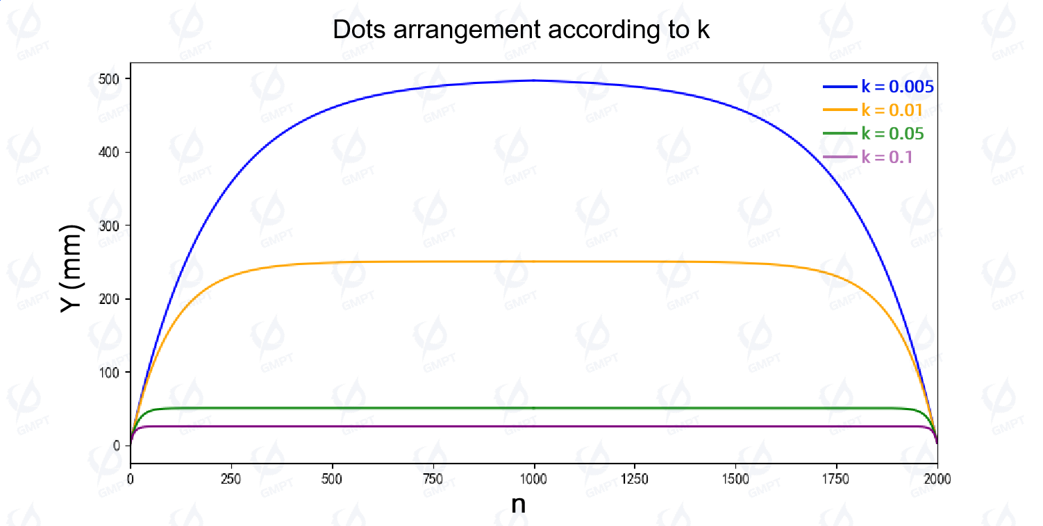
Figure 8 shows the Y-coordinate distribution of dots when adjusting the scattering coefficient ( k ). As light enters the light guide plate from both sides, dot spacing gradually decreases toward the center. When ( k ) increases from 0.005 to 0.1, the distribution transitions from a quadratic function towards a more linear distribution. In theory, polynomial functions can accurately fit various distributions. By adjusting the coefficients of higher-order terms in polynomial arrangements, dot distributions similar to those derived in the theoretical analysis can be achieved.

Figure 8. Dot Distribution with Adjusted \( k \) Parameter

Based on the above analysis, the optimized design parameters for the light guide plate were determined: dot spacing set to 1 mm, radius 0.5 mm, and height 0.1 mm. Compared to a light guide plate without dots—where light is primarily constrained by total internal reflection and circulates within the plate without effective emission—introducing dots disrupts total internal reflection, achieving a more uniform distribution and significantly enhancing light utilization efficiency.

4. Modeling and Simulation of the Backlight Module

4.1 Model Structural Parameter Settings

Table 2. Structural Parameters for the Backlight Module

Components	Length (mm)	Width (mm)	Height (mm)	(x, y, z, α, β, γ)	Material (n, k)	Optical Properties
BEF_I_Prism	162	215	0.025	(0, 3.16, 2.5, 0, 0, 0)	(1.590, 0)	Fresnel_Probabilistic
BEF_I_Substrate	162	215	0.127	(0, 3.084, 2.5, 0, 0, 0)	(1.667, 0)	Fresnel_Probabilistic
BEF_II_Prism	162	215	0.025	(0, 3.34, 2.5, 0, 0, 0)	(1.590, 0)	Fresnel_Probabilistic
BEF_II_Substrate	162	215	0.127	(0, 3.264, 2.5, 0, 0, 0)	(1.667, 0)	Fresnel_Probabilistic
Diffuser	162	215	1	(0, 2.51, 2.5, 0, 0, 0)	PMMA	Fresnel_Probabilistic TopSurface: 85% Scatter_Transmittance
Lightguide	167	222	4	(0, 0, 0, 0, 0, 0)	PMMA	Fresnel_Probabilistic BackSurface/FrontSurface: 99% Specular_Reflection
Reflector	162	215	0.23	(0, -2.12, 2.5, 0, 0, 0)	PMMA	99% Specular_Reflection
Frame_Left	0.95	222	4	(0, 0, -2.45, 0, 0, 0)	NBK7	85% Reflectance
Frame_Right	0.95	222	4	(0, 0, 168.5, 0, 0, 0)	NBK7	85% Reflectance

4.2 LED Light Source Parameter Settings

Table 3. Surface Light Source Parameters

Components	Radiant Power (W)	Length (mm)	Width (mm)	Angular Distribution	Angle from (degree)	Angle to (degree)
White Light	0.38103	3	3	Lambertian	0	60
OGB Light	0.01125	2.8	3.5	Lambertian	0	60

Figure 9. LED Light Spectrum, White Light (left), OGB Colored Light (right)

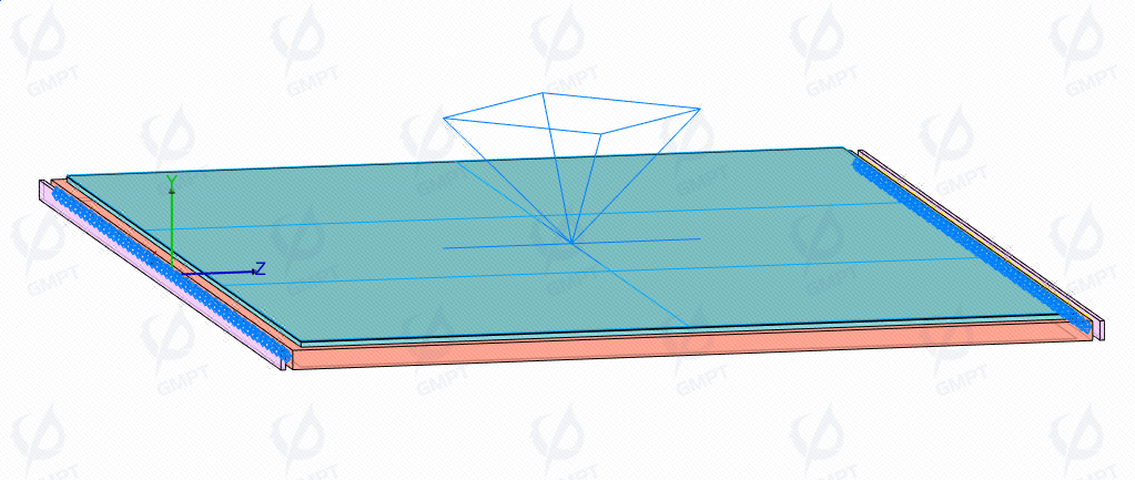
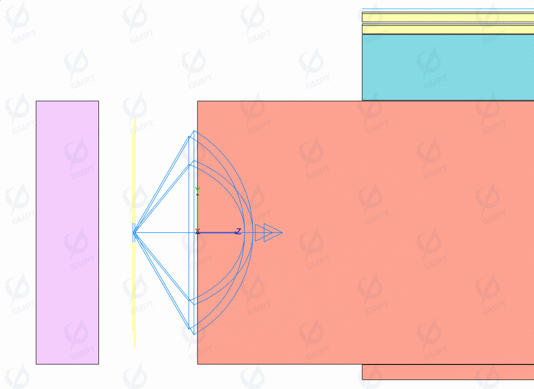
Based on the above configuration, a backlight module model was built, with its visualization shown in Figures 10 and 11, presenting the structure and layout of the model.

Figure 10. Backlight Module Model - Overall Schematic

Figure 11. Side View of the Backlight Module Model

4.3 Simulation Results and Analysis

Using the initial parameters derived from structural analysis (including dot size and spacing on the light guide plate), a simulation analysis of the backlight module model was conducted with 5 million light rays. Figure 12 shows the preview of the light distribution in the model, intuitively displaying the propagation process of the light rays.

Figure 12. Preview of Light Rays in the Backlight Module (100 rays shown in preview)

Figure 13. Illuminance Distribution in Day Mode

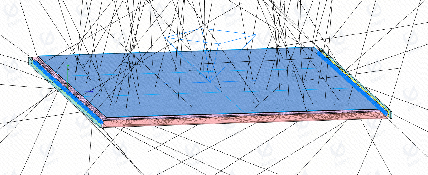
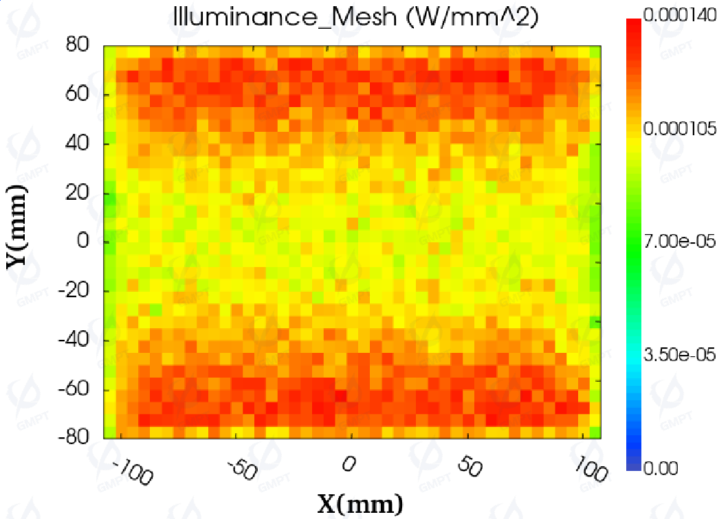
Figure 13 presents the illuminance distribution in day mode, where the illuminance in the region near the receiver is significantly higher than in the central area. This phenomenon results from the matrix uniform arrangement strategy of the dots on the bottom of the light guide plate. When light enters the light guide plate, it reflects off the dots, disrupting the total internal reflection propagation path and entering the receiver. This process reduces energy loss from multiple total reflections, so the light reaching the receiver carries higher power. To further enhance the uniformity of the illuminance distribution, the dot arrangement on the light guide plate was adjusted from a matrix uniform arrangement to a polynomial arrangement strategy. By increasing the texture spacing of the dots on the entry side and shortening the dot spacing in the center region, the goal was to achieve a uniform distribution of light received by the receiver.

$$P(i)=A+\text{sgn}(i)\ast [B\frac{\mathrm{\mid }i\mathrm{\mid }}{N_i}+C{\left(\frac{\mathrm{\mid }i\mathrm{\mid }}{N_i}\right)}^2+D{\left(\frac{\mathrm{\mid }i\mathrm{\mid }}{N_i}\right)}^3+E{\left(\frac{\mathrm{\mid }i\mathrm{\mid }}{N_i}\right)}^4](11)P(i)=A+\backslash text\{sgn\}(i)*\backslash left[B\backslash frac\{|i|\}\{N\_i\}+C\backslash left(\backslash frac\{|i|\}\{N\_i\}\backslash right)^2+D\backslash left(\backslash frac\{|i|\}\{N\_i\}\backslash right)^3+E\backslash left(\backslash frac\{|i|\}\{N\_i\}\backslash right)^4\backslash right]\; \backslash qquad(11)$$

Taking the X direction as an example, where ( P(i) ) represents the position of the dots on the X-axis, ( N_i ) is the normalized index of X, ( A ) is the offset of the first dot from the origin in the X direction; ( B ) represents the uniform arrangement of dots along X; and ( C ), ( D ), and ( E ) are the higher-order coefficients reflecting the trend of densification from the edges to the center of the light guide plate. By adjusting these coefficients, density significantly increases in the center region while the edges are more sparse. When ( B ) is set to 81 and other coefficients to 0, the texture pattern aligns with a uniform matrix arrangement.
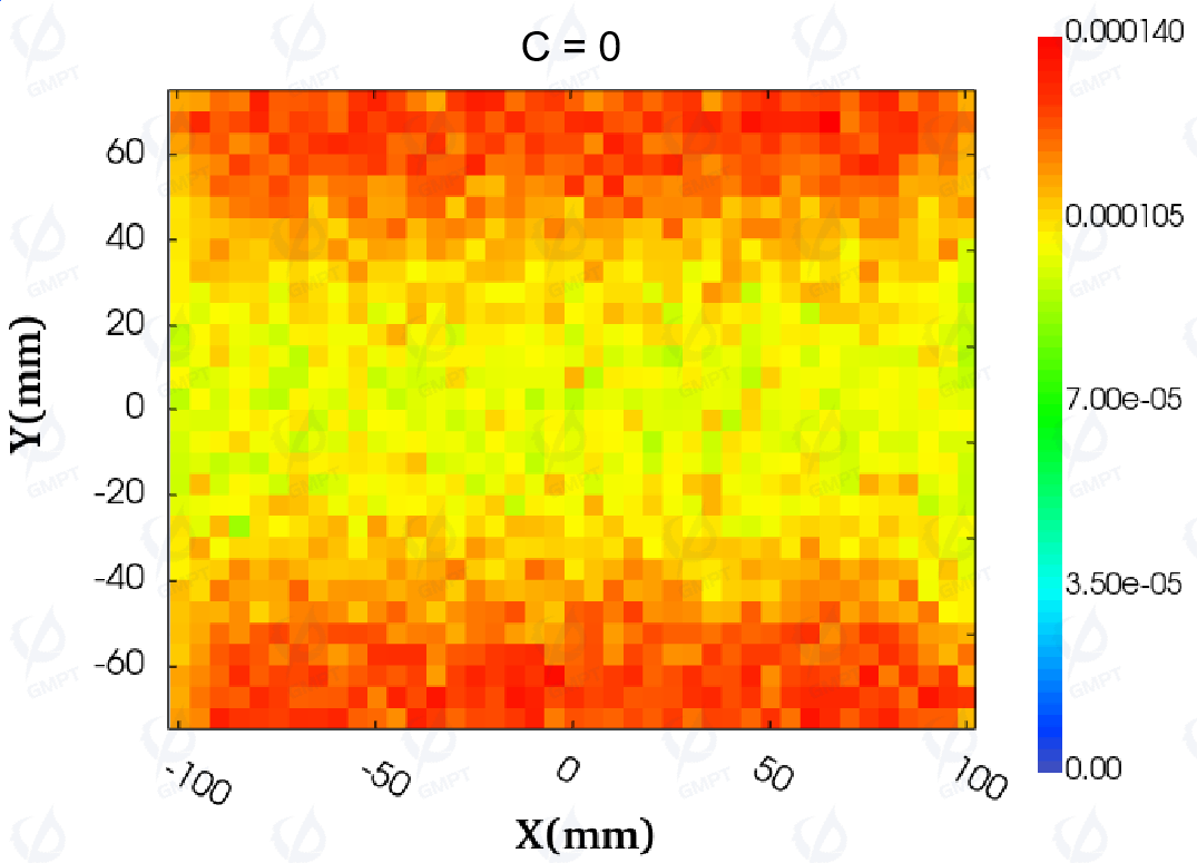
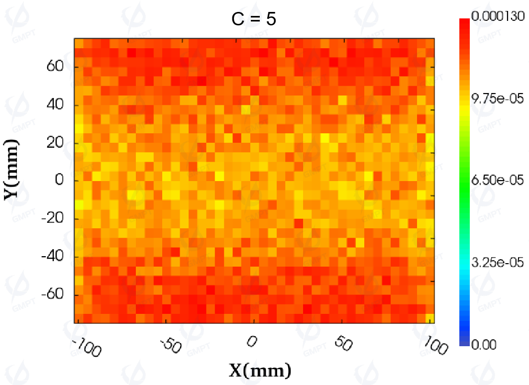
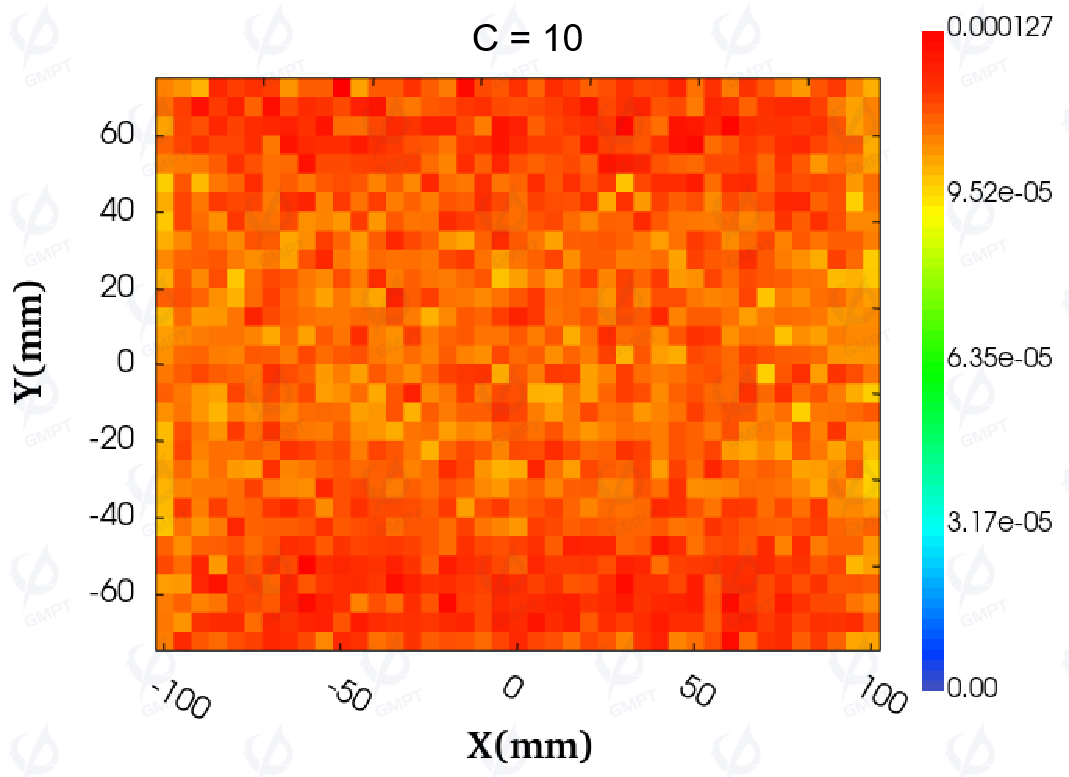
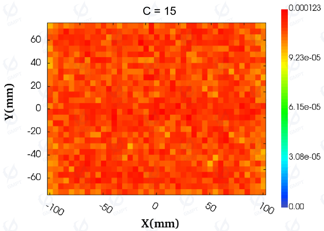
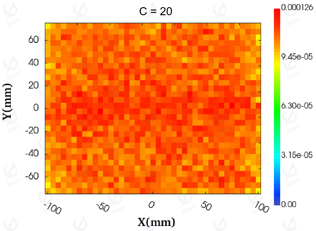
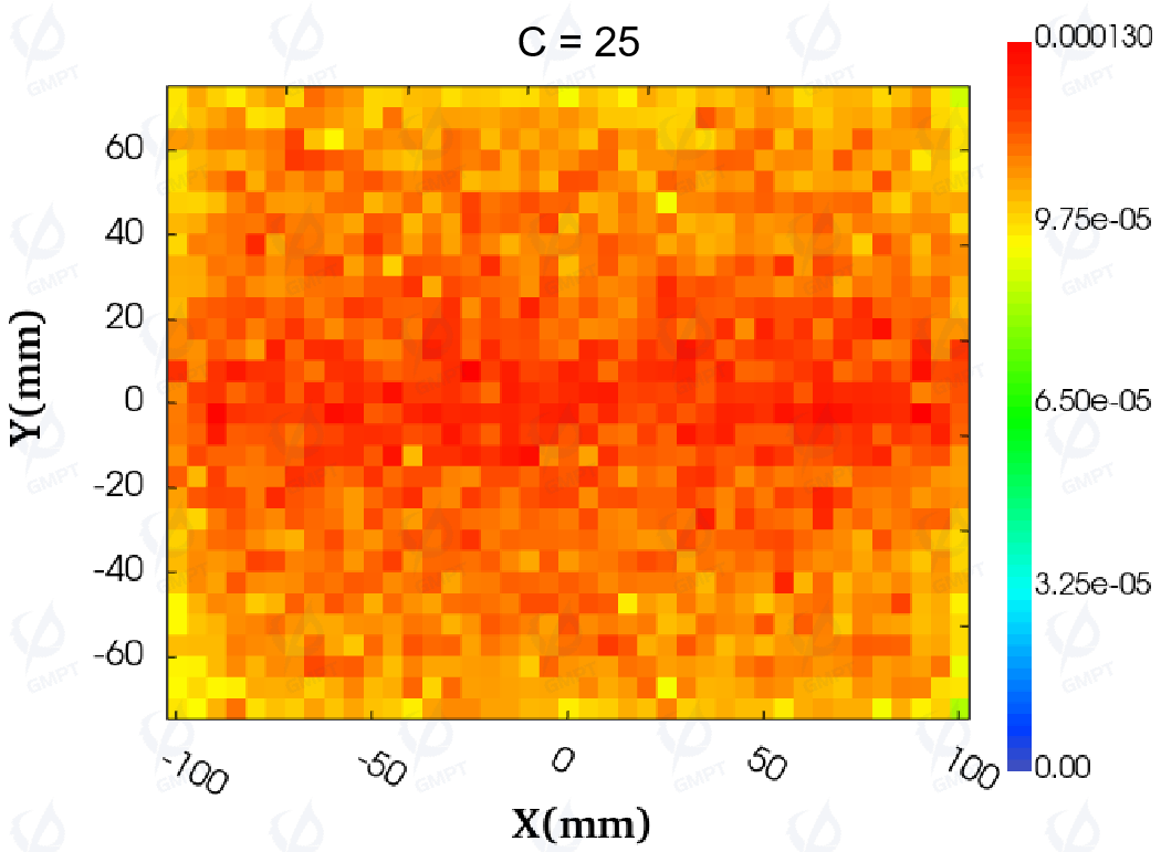
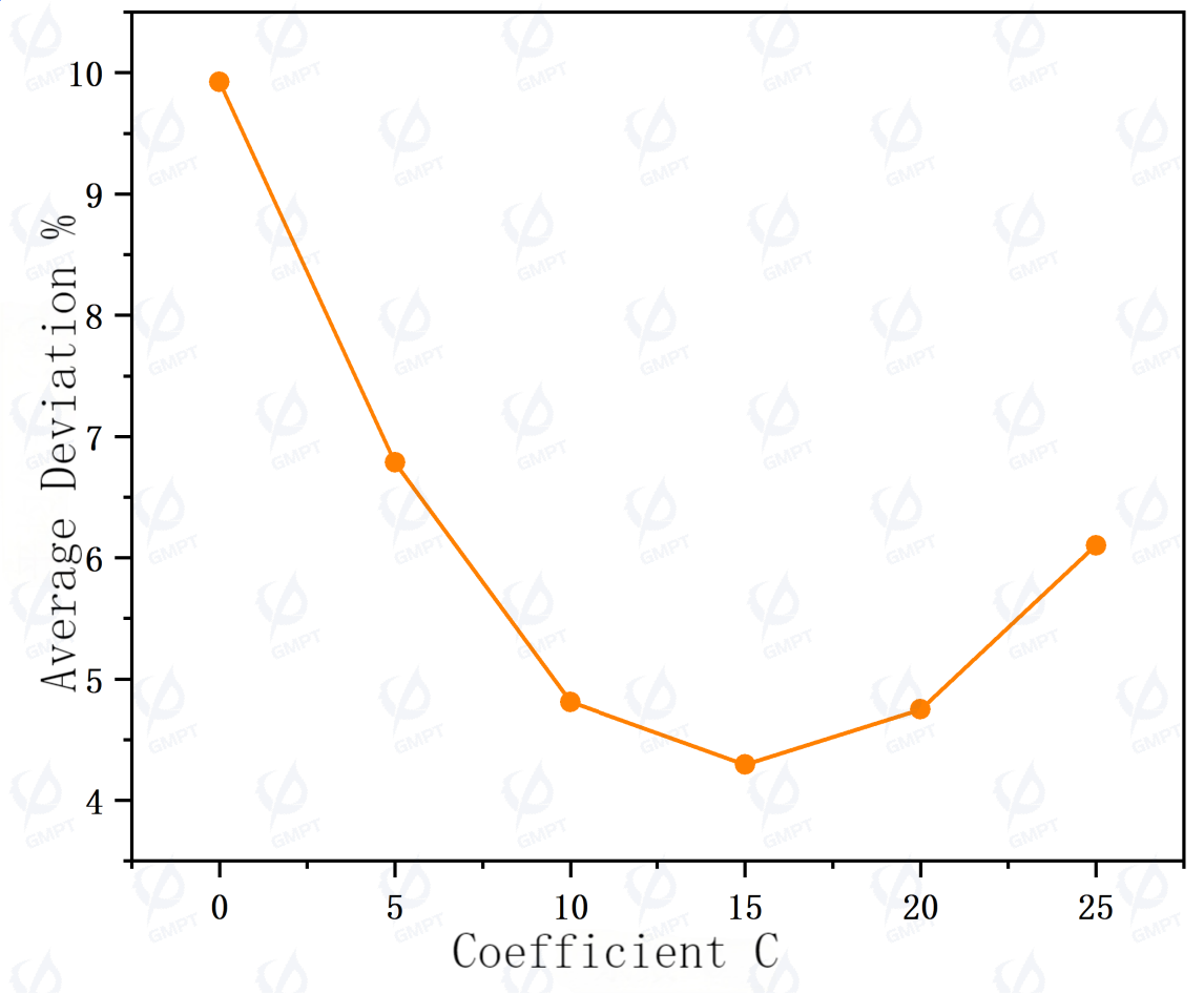
To explore the impact of adjusting the polynomial coefficients on the illuminance distribution, the value of coefficient ( C ) was gradually increased from 0 to 25. Figure 14 visually displays the illuminance distribution before and after adjusting coefficient ( C ). As ( C ) increases from 0 to 20, the distribution shows a relatively uniform state. When ( C ) reaches 25, the distribution changes significantly, with higher illuminance in the middle region and lower values near the light entry side. With ( C ) increasing from 0 to 15, the uniformity of the backlight module's illuminance improves significantly, and the trend aligns with the changes in illuminance distribution and uniformity.

Figure 14. Illuminance Distribution with Adjusted Polynomial Coefficient \( C \) in Day Mode

The contrast ratio (non-uniformity) is calculated as follows:

$$\text{Contrast Ratio}=\frac{\text{max}-\text{min}}{\text{max}+\text{min}}(12)\backslash text\{Contrast\; Ratio\}\; =\; \backslash frac\{\backslash text\{max\}\; -\; \backslash text\{min\}\}\{\backslash text\{max\}\; +\; \backslash text\{min\}\}\; \backslash qquad(12)$$

where the Contrast Ratio represents the illuminance non-uniformity of the backlight module; max is the maximum illuminance, and min is the minimum illuminance of the backlight module.

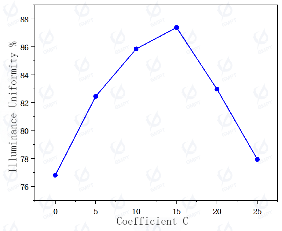
Figure 15 further presents the trend graphs of illuminance uniformity and average deviation calculated using the non-uniformity formula. When the coefficient ( C ) is set to 15, the illuminance uniformity of the backlight module improves to 87.40% (meeting practical uniformity requirements), and the average deviation reaches a minimum value of 4.29%. These data indicate the effectiveness of coefficient adjustment in optimizing the uniformity of the backlight module's illuminance.

Figure 15. Illuminance Uniformity Trend (left) and Average Deviation Trend (right) in Day Mode

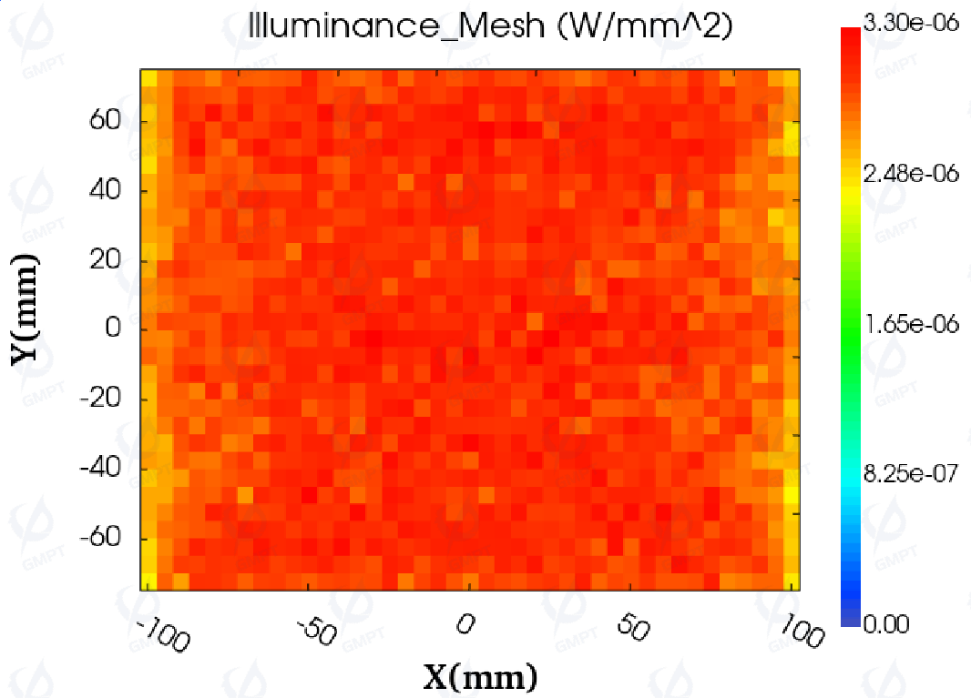
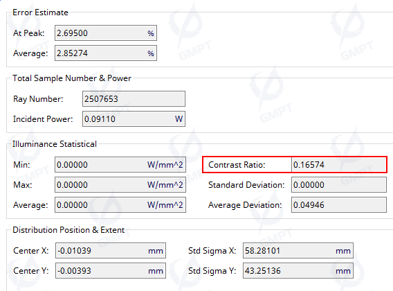
Using the adjusted parameters for the dots on the light guide plate, the simulation results for the backlight module in night mode are shown in Figure 16. In night mode, the contrast ratio result is 16.574%, so the illuminance uniformity is 83.426%, with an average deviation of 4.946%, also meeting practical uniformity requirements.

Figure 16. 2D Illuminance Distribution in Night Mode (left) and Statistical Information (right)

5. Summary

This paper first introduces the background and structural composition of the night vision-compatible LCD backlight module. Subsequently, the model structure parameters of the backlight module were initially determined based on a dual-mode light source strategy and optimized dot layout for the light guide plate. Then, based on simplified model calculations, the optimal dot distribution was computed. By analyzing the trend of non-uniformity in the illuminance distribution of the simulation results, the dot arrangement was adjusted from a matrix uniform layout to a polynomial layout strategy. Finally, using these structural data, illuminance uniformity simulations were conducted for day and night modes, and the results show that they meet practical uniformity requirements.
Future work will focus on refining dot arrangement patterns, specifically strategies such as AI-adjusted polynomial coefficients and list arrangement methods, to precisely control the spacing of the dots on the light guide plate. These optimizations aim to enhance the overall illuminance uniformity of the backlight module, achieving a more balanced and efficient lighting effect.

References

1. Zhu, Xiangbing, et al. "Research on LED LCD Backlight Module Compatible with Night Vision." Laser & Optoelectronics Progress, vol. 54, no. 09, 2017, pp. 207-211.
2. Li, Zhengrong, et al. "Analysis of Night Vision Compatibility in LED Backlight LCDs." Laser & Optoelectronics Progress, vol. 51, no. 05, 2014, pp. 186-192.
3. Chang, Yunfei. "Research on LED Backlight Compatible with Night Vision in LCDs." Master’s Thesis, Hefei University of Technology, 2013.
4. Jiao, Yao. "Design and Research of Backlight Module for On-board LCD Modules." Master’s Thesis, Anhui Normal University, 2018.
5. Wang, Yongwu. "Optimization Design of Scattering Dots in Edge-lit Light Guide Plates and Laser Processing Technology." Master’s Thesis, Qingdao University of Technology, 2019.
6. Lin, Xiaoxin, et al. "Design and Simulation of Dots in Edge-lit LED Backlight Guide Plates." Journal of Guangdong University of Technology, vol. 31, no. 04, 2014, pp. 95-99.