Henyey-Greenstein Volume Scattering

  Henyey-Greenstein is one of the simplest and most common models used to describe light scattering within materials. It is often applied in simulation cases for atmospheric and life sciences. The Henyey-Greenstein scattering model, proposed by Henyey and Greenstein in 1941, is empirical rather than based on electromagnetic principles. Due to its simplicity and flexibility, the HG phase function is a useful tool for simulating various scattering properties, helping scientists and engineers better understand and model the interaction of light with materials.

  An important parameter in volume scattering is the Mean Free Path (MFP), representing the expected distance light travels within a material before scattering occurs. The reciprocal of MFP is the scattering coefficient, which represents the expected number of scattering events per unit distance. The default value of MFP is usually set to infinity. The MFP Scaled Factor is a coefficient used to adjust the MFP, often applied in scenarios where particle concentration varies. It is inversely proportional to particle concentration, reflecting the relationship where higher particle concentrations result in shorter mean free paths.   The relationship between the scaled $MFPMFP$ and the original $MFPMFP$ is:

$$\text{Scaled MFP}=\text{MFP}\times \text{MFP Scaled Factor}\backslash text\{Scaled\; MFP\}\; =\; \backslash text\{MFP\}\; \backslash times\; \backslash text\{MFP\; Scaled\; Factor\}$$

  Scattering is a Poisson process, meaning the probability of scattering at any given point is uniform. The probability density function (PDF) of the Henyey-Greenstein phase function is:

$$p(\mu )=\frac{1}{2}\frac{1-g^2}{{[1+g^2-2g\mu ]}^{3\mathrm{/}2}}p(\backslash mu)\; =\; \backslash frac\{1\}\{2\}\; \backslash frac\{1-g^2\}\{\backslash left[1+g^2-2g\backslash mu\backslash right]^\{3/2\}\}$$

  The cumulative distribution function $FF$ for scattering can be calculated as:

$$F(x,{\sigma }_s)={\int }_0^x{\sigma }_s{e}^{-{\sigma }_{s}t}dtF(x,\; \backslash sigma\_s)\; =\; \backslash int\_0^x\; \backslash sigma\_s\; e^\{-\backslash sigma\_s\; t\}\; \backslash ,\; dt$$

Resulting in:

$$F(x,{\sigma }_s)=1-e^{-{\sigma }_{s}x}F(x,\; \backslash sigma\_s)\; =\; 1\; -\; e^\{-\backslash sigma\_s\; x\}$$

  The inverse function of $FF$ provides the free path $xx$:

$$x=-\text{MFP}\cdot \ln (1-F)x\; =\; -\backslash text\{MFP\}\; \backslash cdot\; \backslash ln(1-F)$$

  By sampling a random number $FF$ in [0,1], we can determine the free path of light. Comparing this free path to the distance to the surface determines if scattering occurs, guiding the decision to perform volume scattering sampling.

  The sampling direction of scattering is determined by the Henyey-Greenstein phase function:

$$P(\theta )=\frac{1-g^2}{4\pi (1+g^2-2g\cos \theta {)}^{1.5}}P(\backslash theta)\; =\; \backslash frac\{1-g^2\}\{4\backslash pi(1+g^2\; -\; 2g\backslash cos\backslash theta)^\{1.5\}\}$$

  In Henyey-Greenstein scattering, the scattering angle depends on the anisotropy parameter $gg$ in [-1,1]:

• $gg$ > 0: Forward scattering.
• $gg$ = 1: No scattering (perfect forward direction).
• $gg$ < 0: Backward scattering. Specifically, when $g=-1g=-1$, the light undergoes complete backward scattering.
• $gg$ = 0: Isotropic scattering (equal probability in all directions).

Therefore, in the absence of volume scattering, the default value of $𝑔𝑔$ is typically set to 1.

  Since the Henyey-Greenstein model is an empirically derived scattering model, the value of $gg$ can typically be fitted in real-world scenarios using the following formula:

$$g_1={\int }_0^{2\pi }{\int }_0^{\pi }P(\theta )\cos \theta \sin \theta d\theta d\varphi g\_1\; =\; \backslash int\_0^\{2\backslash pi\}\; \backslash int\_0^\backslash pi\; P(\backslash theta)\; \backslash cos\backslash theta\; \backslash sin\backslash theta\; d\backslash theta\; d\backslash phi$$

  This value represents the expected cosine of the scattering angle.
  The particle transmissivity defines the relative power loss during scattering, given by:

$$P^{\mathrm{\prime }}=P\times TP\text{'}\; =\; P\; \backslash times\; T$$

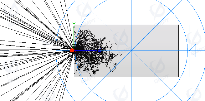
  In practice, Henyey-Greenstein scattering is often used to plot backscatter curves for similarity analysis. The typical setup includes a red point source and a surrounding blue spherical far-field detector:

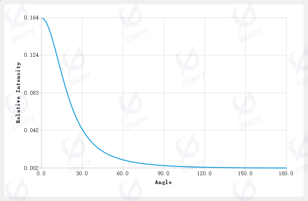
  The Henyey-Greenstein backscatter curve describes the directional distribution of scattered light, where:

• $xx$-axis: Scattering angle $\theta \backslash theta$. This angle represents the angle between the incident light and the scattered light, ranging from 0° to 180° (0° for forward scattering, 180° for backward scattering).
• $yy$-axis: Scattering intensity or probability , given by the phase function $P(\theta )P(\backslash theta)$.

  To enhance the simulation experience, Rayzen provides:

1. Basic Henyey-Greenstein volume scattering ray tracing, allowing for direct specification of parameters such as mean free path, anisotropy factor, and particle transmissivity, or indirect specification of related parameters (e.g., scattering coefficient, reduced scattering coefficient, and scaled mean free path). This enables simulation of the phenomena occurring when light passes through objects containing particles modeled by the Greenstein model.

2. Quick preview functionality for theoretical scattering parameter calculations at specified wavelengths for materials, including viewing scattering curves, interpolating other related parameters from the above examples, and performing calculations and visualizations.

3. Tracking and highlighting the scattering trajectory of individual rays, along with auxiliary features such as rendering surrounding objects as transparent.

  We first define a sample object for scattering with the following properties such as the location and geometric information:

Geometry Type	Radius	Height	Taper	(x, y, z, α, β, γ)
Cylinder	5 mm	20 mm	1	(0, 0, 0, 0, 0, 0)

  All surfaces are defined with perfect_transmitter optical properties.
  The material is a gas sample with refractive index 1 and transmissivity 1, containing particles modeled using Henyey-Greenstein scattering.The cylindrical material is a gas sample with a refractive index of 1 and a transmissivity of 1, containing particles modeled using the Greenstein scattering model. After setting the material type to isotropic and the particle volume scattering type to Henyey-Greenstein, the scattering properties can then be configured.   The scattering properties are configured as follows:

We support three methods for defining MFP: direct input, scattering coefficient, or reduced scattering coefficient. Here, we simply choose to input the mean free path directly. The scaling factor for the mean free path is set to the default value of 1. The table of input wavelengths and mean free paths is as follows:

Wavelength (nm)	Mean Free Path (mm)
545	0.08
555	0.12

The table of input wavelengths and anisotropic parameters is as follows:

Wavelength (nm)	Anisotropy Factor
540	0.7
560	0.6

The table of input wavelengths and particle transmissivity is as follows:

Wavelength (nm)	Particle Transmissivity
555	0.8

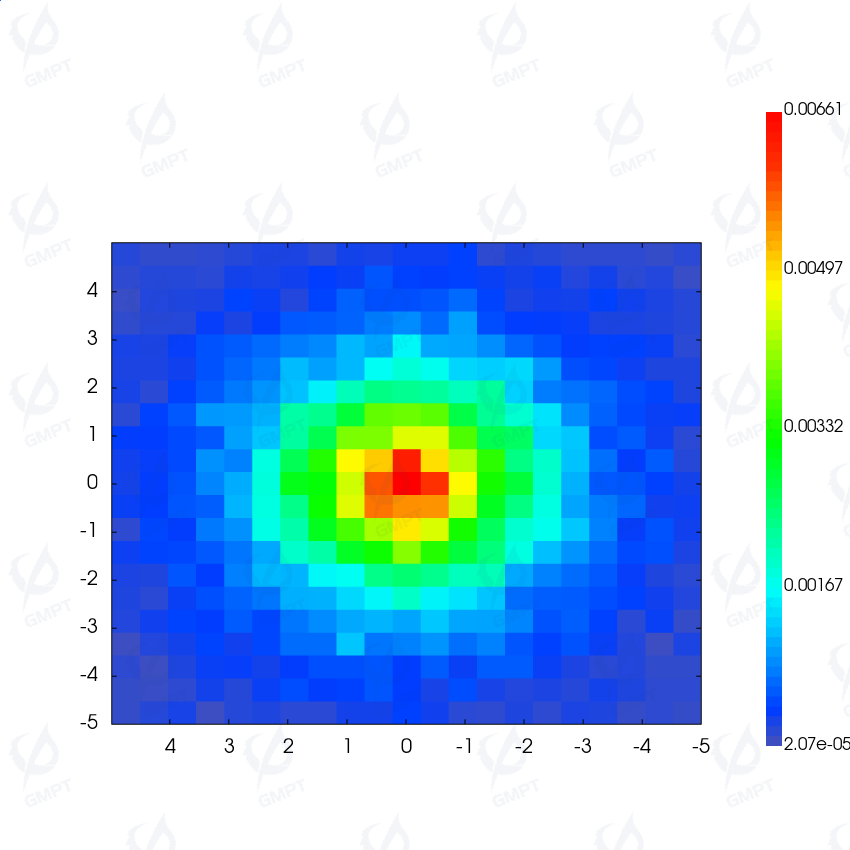
  The results from the planar detector are shown below:

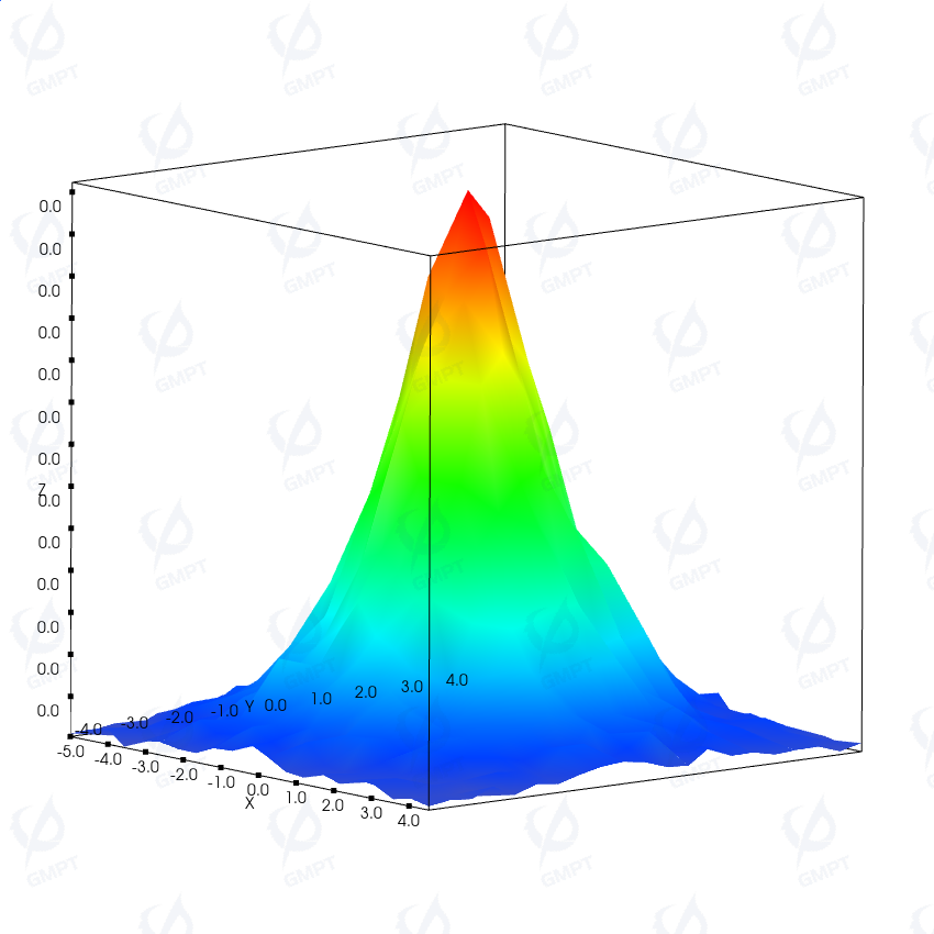
  The 3D representation of illuminance is shown below while the vertical axis represents the illuminance magnitude:

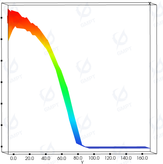
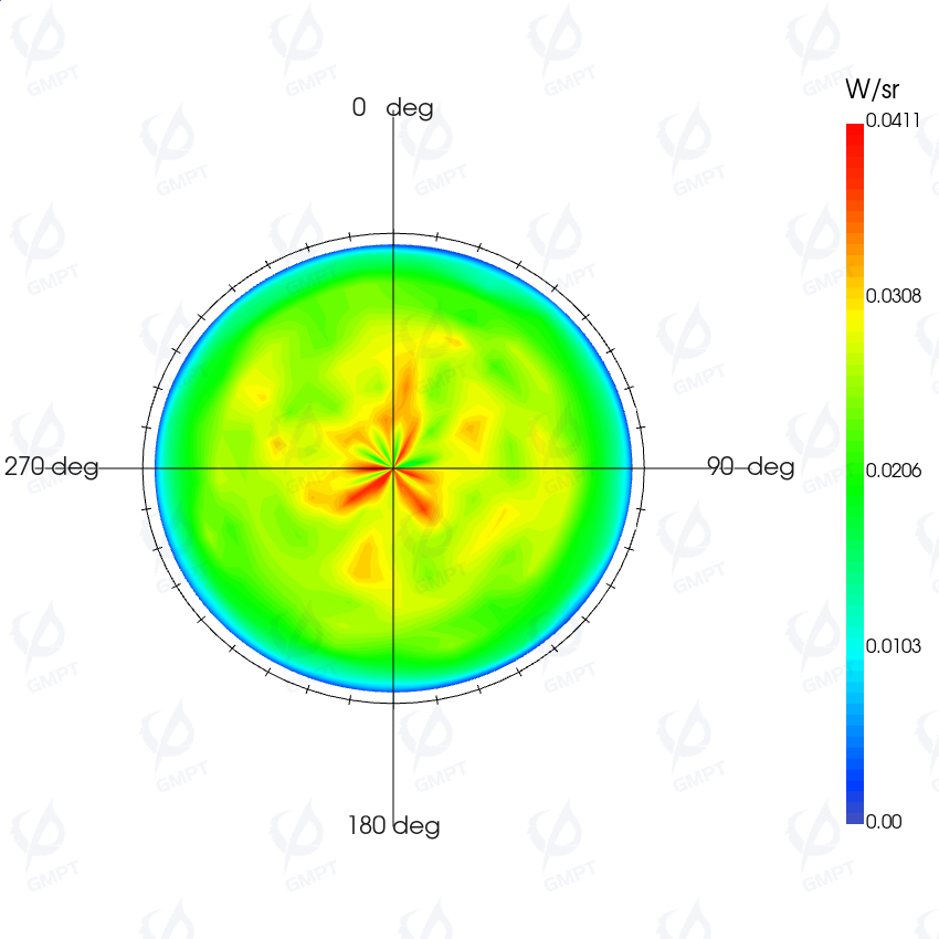
  The far-field detector's results:

  At 550 nm, the scattering curve parameters are:

Property	Value
Wavelength	550 nm
Mean Free Path	0.1 mm
Scatter Coefficient	10
Reduced Scatter Coeff.	4
Average Cosine	0.65
Gamma	1.65

  According to Greenstein's definition of the scattering anisotropy parameter, when the scattering angle is 0 degrees, the central region typically exhibits the highest scattering probability.

  The phase function curve for 550 nm:

  After simulating 100,000 rays, we can obtain the actual scattering curve from the side view of the 3D Cartesian coordinate plot:

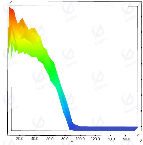
  After increasing ray count to 1,000,000 for achieving a more convergent and smoother result: