Reverse Design of Y-branch Optical Waveguide Devices

GMPT, October 2024

Traditional photonic device design is based on the physical principles of the device and is optimized through numerical simulation. This approach is limited by predefined models, offering restricted design freedom. To meet the demand for high-performance devices, reverse design methods with higher degrees of freedom have rapidly developed. Reverse design explores the entire parameter space to find the optimal solution, enabling the design of devices with superior performance.
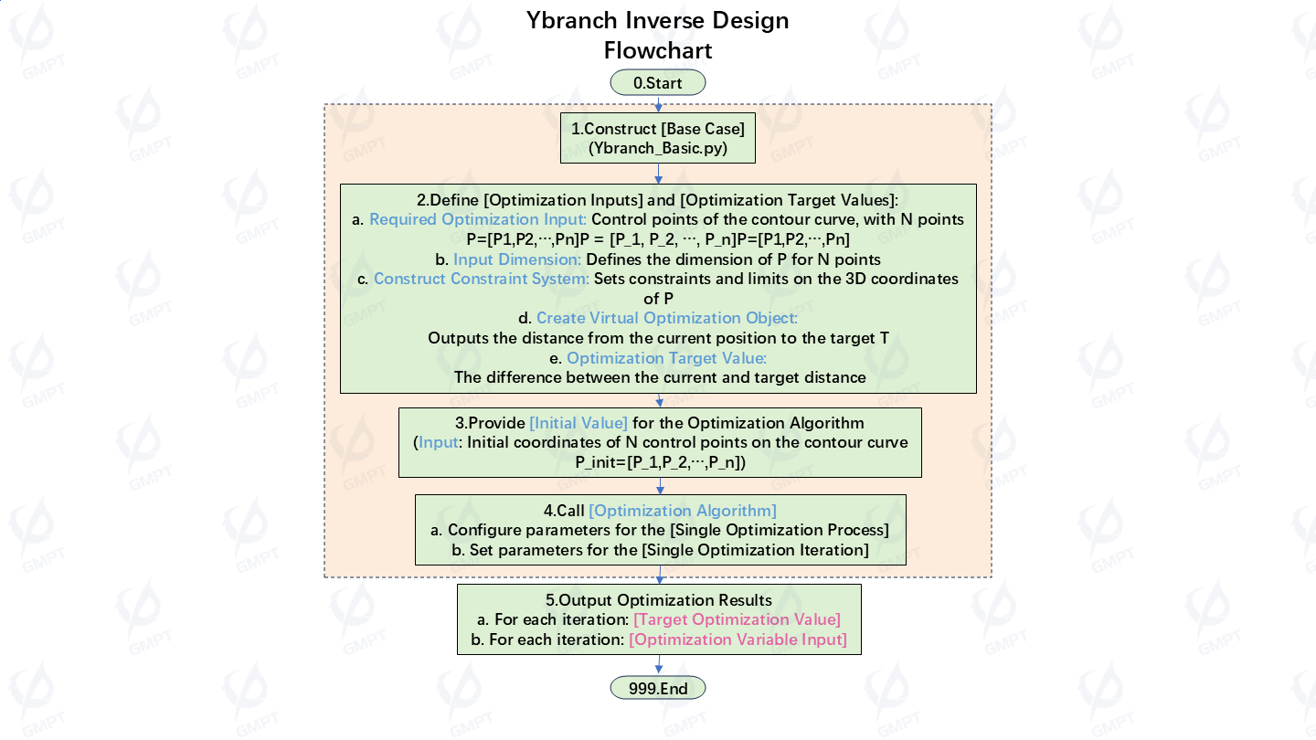
This article uses Macondo to establish a reverse design model for Y-branch optical waveguide devices. The Nelder-Mead and Genetic algorithms are employed to optimize the Y-branch waveguide profile and achieve the best transmission efficiency. The flowchart below illustrates the reverse design process of Y-branch devices using optimization algorithms.

Figure 1. Y-branch reverse design flowchart

1. Introduction to the Reverse Design Device Structure

Y-branch waveguide devices are primarily used in integrated optical circuits for splitting (splitter mode), combining (combiner mode), or both functions (bidirectional mode). These devices have extensive applications in optical power splitters, optical switches, and Mach-Zehnder modulators.
In this simulation case, the Y-branch device is used in splitter mode, where light enters through a single input port and exits through two output ports. The waveguide structure connecting the input and output ports is optimized to ensure that the total power of the two output waveguides is as close as possible to the input power.

1.1 Initial Conditions of the Device Structure

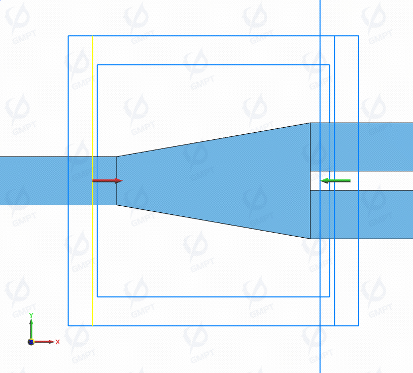
The Y-branch device in this simulation uses Si material enclosed in an SiO₂ region. The input and output rectangular waveguides are each $3 u m$ in length, $0.5 u m$ in width, and $0.22 u m$ in thickness, with an output waveguide spacing of $0.7 u m$ . The waveguide structure between the input and output ports uses a polygonal geometry where vertices are connected to form a tapered structure. This serves as the initial profile for the Y-branch design. Below is the initial structure of the Y-branch device.

Figure 2. Initial structure of the Y-branch device

1.2 Definition of the Profile Line Function

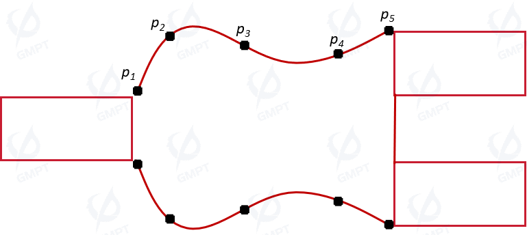
In this case, the Y-branch profile is defined using cubic spline interpolation. Based on a set of $x$ -positions, $n$ control points are generated to construct a smooth curve. Figure 3 shows a curve constructed using cubic spline interpolation, marking the control points. More control points allow for finer adjustments to the overall shape by reducing the radius of curvature. However, manufacturing processes limit the minimum feature size, and optimizing many control points significantly increases simulation time.

Figure 3. Cubic spline interpolation curve as a Y-branch profile

Cubic spline interpolation constructs a series of cubic polynomial segments to approximate data points while ensuring continuity in the first and second derivatives, resulting in a smooth interpolation function. Polynomial coefficients are determined by solving a system of linear equations to achieve smooth transitions between data points.
The process is implemented using splrep from scipy.interpolate. Example code:

def get_pts(ys):
    global x_min, x_max, y_min, y_max
    xs = [x_min]
    for i in range(1, intervals):
        xs.append(x_min + i / intervals * (x_max - x_min))
    xs.append(x_max)
    ys.insert(0, y_min)
    ys.append(y_max)
    tck = interpolate.splrep(xs, ys)
    x_points, y_points = [], []

Interpolated curve sampling points are extracted and used as vertices of the profile polygon, forming the polygonal structure needed for simulation. Example code:

for i in range(101):
    x = x_min + i / 100 * (x_max - x_min)
    y = interpolate.splev(x, tck)
    x_points.append(x)
    y_points.append(y)

In this case, the $x$ -coordinate interval is divided into 10 control points as optimization variables for smooth profile transitions. The $y$ -coordinate is restricted to $0.2 μ m$ to $0.8 μ m$ to ensure design feasibility.

1.3 Optimization Goal

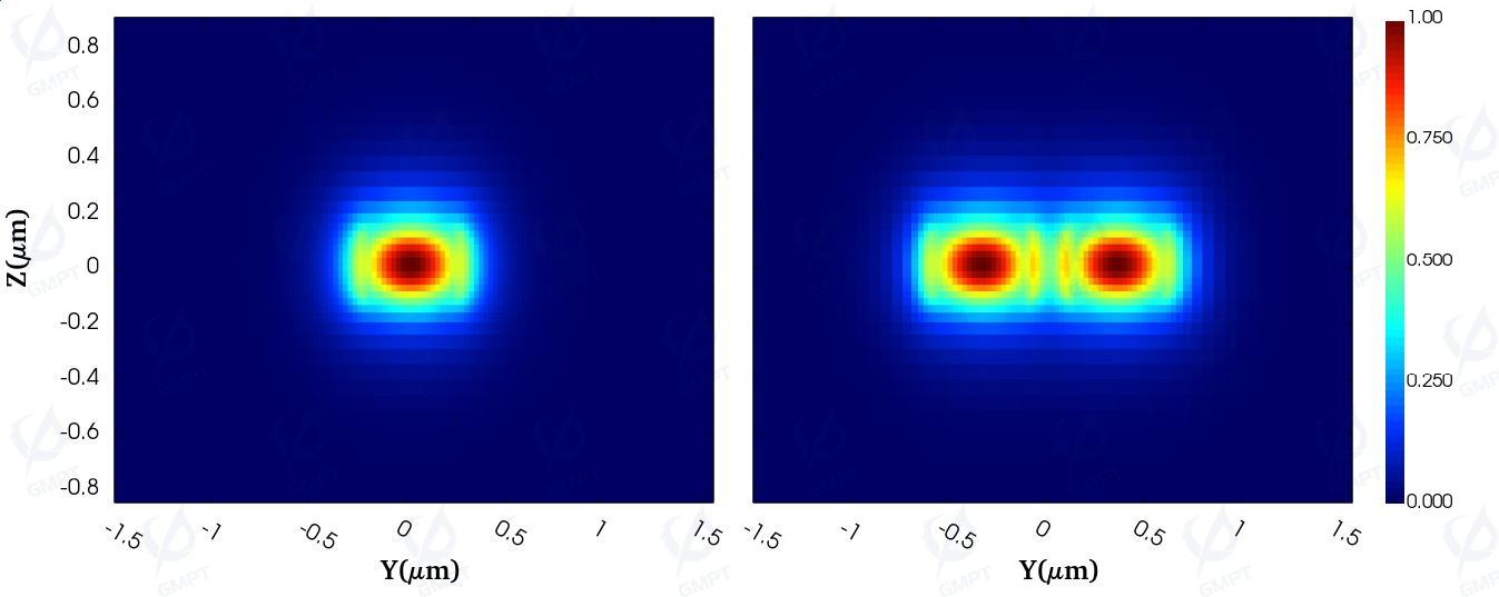
The optimization simulation uses a $1.55 μ m$ mode light source. The mode expansion algorithm calculates the transmission power ratio at the output waveguides, and the difference between this transmission and the target value is the optimization objective. The field distribution at the two output ports is shown below. The ideal output power ratio to the input power is 1, representing the target transmission efficiency.

Figure 4. Mode distribution at two Y-branch output ports

Next, optimization algorithms iterate on the objective function to find the best solution and optimal function value within the given iterations.

2. Optimization of Device Structure Using the Nelder-Mead Algorithm

The Nelder-Mead algorithm is a gradient-free optimization method that iteratively updates the simplex polytope formed by vertices. It employs operations such as reflection, expansion, and contraction to approximate the minimum point in multidimensional space.

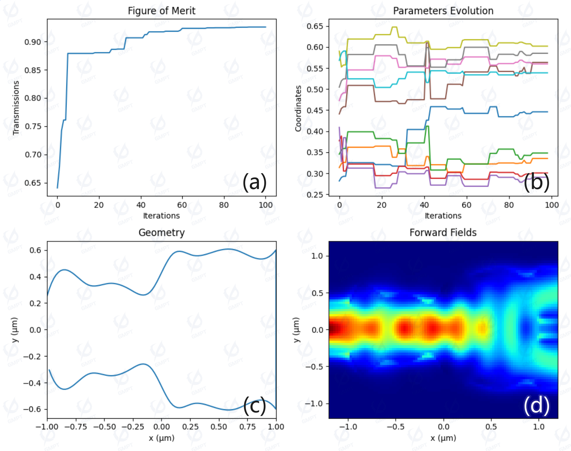
Figure 5. Results of Nelder-Mead reverse design: a) Iterative process of optimizing transmission efficiency b) Variation of profile control points during iterations c) Optimized device profile d) Optimized power distribution

In this case, since the objective function involves simulation calls, evaluating the objective function is computationally expensive. As the Nelder-Mead method requires fewer function calls per iteration, its runtime is relatively short. Figure 5a shows the device transmission efficiency stabilizing at approximately ( 92% ) after 100 iterations. Figure 5b shows the changes in the profile control points during iterations. Figures 5c–5d show the profile and field distribution obtained using the Nelder-Mead algorithm.

3. Optimization of Device Structure Using the Genetic Algorithm

The Genetic Algorithm is a heuristic search method that simulates natural selection and genetic mechanisms to solve optimization problems. It encodes potential solutions as chromosomes and explores the solution space through genetic operations such as selection, crossover, and mutation. Individuals with better performance in each generation are more likely to be selected to produce the next generation, gradually approaching the optimal solution.

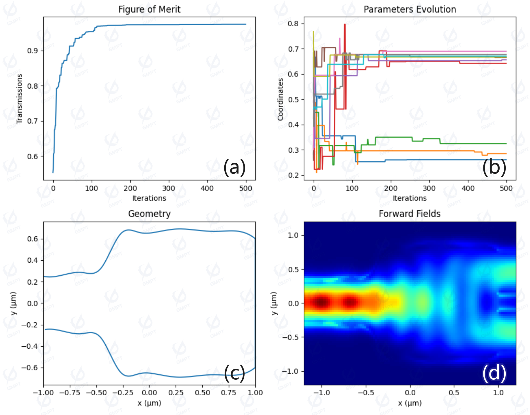
Figure 6. Results of Genetic Algorithm reverse design: a) Iterative process of optimizing transmission efficiency b) Variation of profile control points during iterations c) Optimized device profile d) Optimized power distribution

However, the Genetic Algorithm requires more simulation calls per iteration (e.g., 10 calls for 10 optimization variables), making it slower than the Nelder-Mead algorithm. Figure 6a shows the device transmission efficiency reaching approximately $96$ % after 100 iterations and $97.5$ % after 200 iterations. Figure 6b shows the changes in the profile control points during iterations. Figures 6c–6d show the profile and field distribution obtained using the Genetic Algorithm.

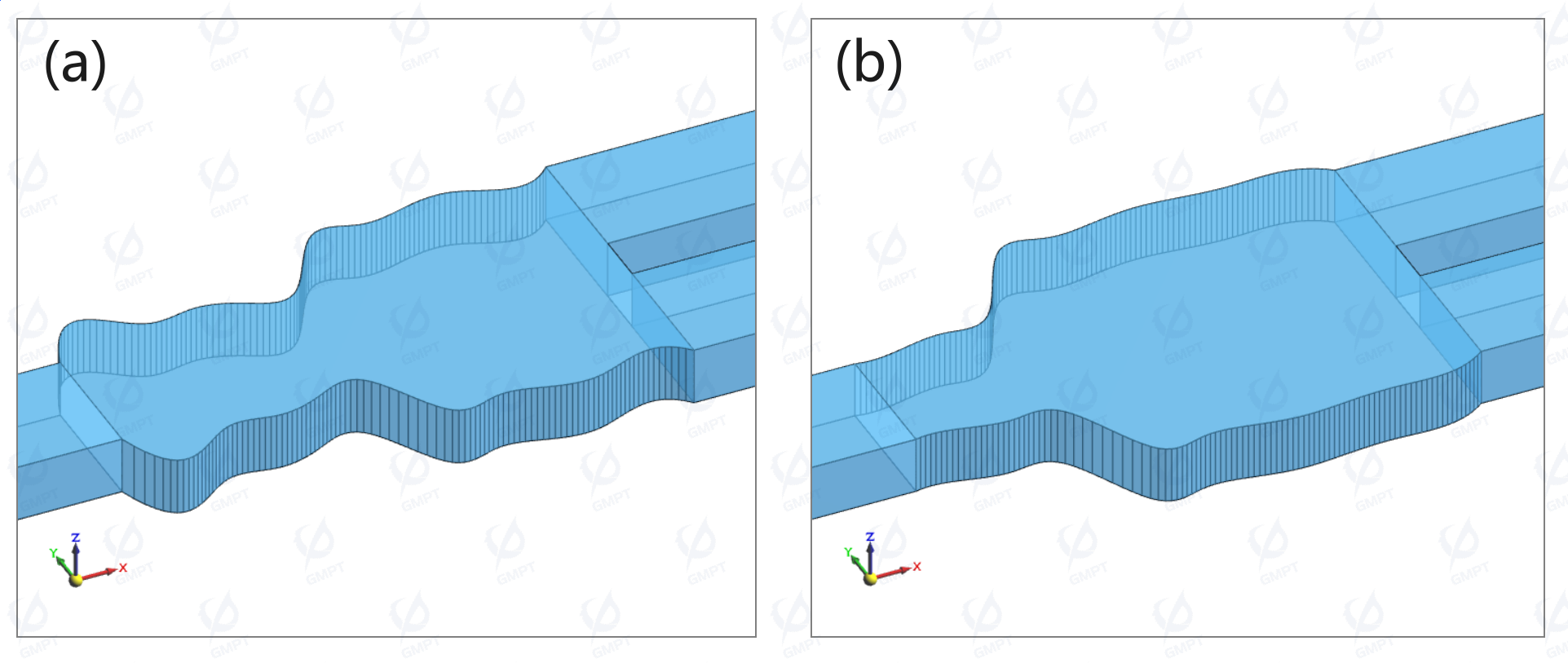
Finally, the complete device structure obtained through reverse design using Macondo is shown below.

Figure 7. Final Y-branch device structures: a) Nelder-Mead b) Genetic Algorithm

4. Conclusion

This article introduces the reverse design process of Y-branch devices using optimization algorithms. The device profile curve was constructed with cubic spline interpolation, and the Nelder-Mead and Genetic Algorithms were used to optimize the structure for high transmission efficiency. Future work will explore neural network-based reverse design methods and the adjoint method to improve the efficiency of Y-branch device reverse design simulations.

References

[1] Hsu C W, Chen H L, Wang W S. Compact Y-branch power splitter based on simplified coherent coupling[J]. IEEE Photonics Technology Letters, 2003, 15(8): 1103-1105.
[2] Inverse design of y-branch – Ansys Optics
[3] Optimization (scipy.optimize) — SciPy v1.14.1 Manual